One Zero Blog

Article Outline

• Data Background
• Aim of the modelling
• Data Loading
• Basic Exploratory Analysis
• Multiple Linear Regression Model Fitting/Estimation
• Interpretation of MLR Model Summary
• Binary Logistic Regression Model Fitting/Estimation
• Interpretation of the Logistic Regression Model Summary
• References
• Dataset and Code

Data Description

The dataset contains several parameters which are considered important during the application for Masters Programs. The parameters included are as follows:

• I1: GRE Scores ( out of 340 )
• I2: TOEFL Scores ( out of 120 )
• I3: University Rating ( out of 5 )
• I4: Statement of Purpose Strength ( out of 5 )
• I5: Letter of Recommendation Strength ( out of 5 )
• I6: Undergraduate GPA ( out of 10 )
• I7: Research Experience ( either 0 or 1 )
• O: Chance of Admit ( ranging from 0 to 1 )

I: independent variable; O: outcome variable

Inspiration

This dataset was built with the purpose of helping students in shortlisting universities with their profiles [2]. The predicted output gives them a fair idea about their chances for a particular university.

Dataset Link: https://www.kaggle.com/mohansacharya/graduate-admissions

Aim of the Article

The aim of this article is to fit and interpret a Multiple Linear Regression and Binary Logistic Regression using Statsmodels python package similar to statistical programming language R. Here, we will predict student admission in masters’ programs. Additionally, we will learn how we could interpret the coefficients obtained from both modelling approaches.

Loading Libraries

The very first step is to load the relevant libraries in python.

import numpy as np                 # Array manipulation
import pandas as pd                # Data Manipulation
import matplotlib.pyplot as plt    # Plotting
import seaborn as sns              # Advanced statistical plotting

# MLR and Logistic Regession model fitting
import statsmodels.api as sm       
from statsmodels.formula.api import ols, logit

# VIF computation
from statsmodels.stats.outliers_influence import variance_inflation_factor

Loading data

Let’s read the “Admission” dataset using pandas read_csv( ) function and print first 5 rows.

admission = pd.read_csv("Admission.csv")
admission.head()

Next, let’s check the column names using the .column attribute.

admission.columns

Descriptive Statistics

Before proceeding to the modelling part, it is always a good idea to get familiar with the dataset. An exploratory analysis could help in this regard. To obtain the data set information we can use the .info( ) method. The dataset has 400 observations and 8 columns which consist of integers and floats.

admission.info()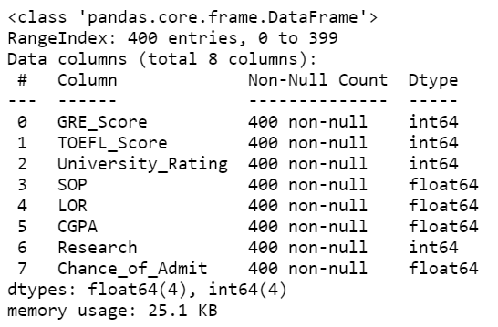

We can check the descriptive statistics of the dataset using .describe( ) attribute.

admission.describe()

The next step will be to explore the relationship between different variables.

Scatter Plot Matrix

Here, I have plotted a scatter plot matrix to explore the relationship between different variables. The matrix diagonal presents distribution of variables (histogram).

sns.pairplot(admission, vars = ['GRE_Score', 'TOEFL_Score', 'University_Rating', 'SOP', 'LOR', 'CGPA', 'Chance_of_Admit'])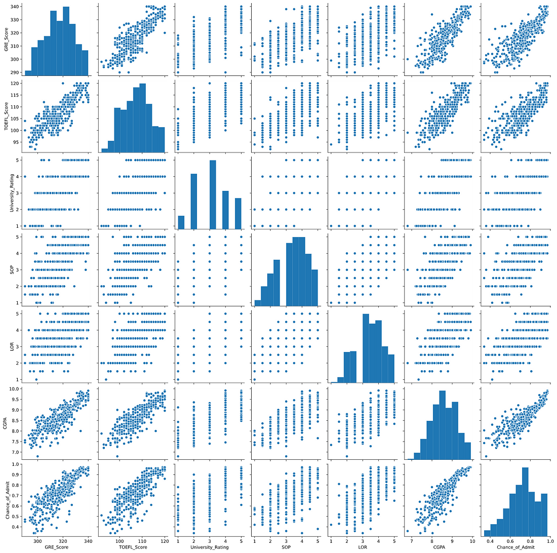

Multicollinearity Check

Before we proceed to MLR or logistic regression we need to check one assumption that the independent variables (predictors) should be free from any correlation. The rule of thumb that the inter-predictor correlation should be <0.4. To understand the correlation between predictors we can estimate the correlation matrix and plot it using matplotlib library.

corr = admission.corr()
fig, ax = plt.subplots(figsize=(10, 8))
colormap = sns.diverging_palette(220, 10, as_cmap = True)
dropvals = np.zeros_like(corr)
dropvals[np.triu_indices_from(dropvals)] = True
sns.heatmap(corr, cmap = colormap, linewidths = .5, annot = True, fmt = ".2f", mask = dropvals)
plt.show()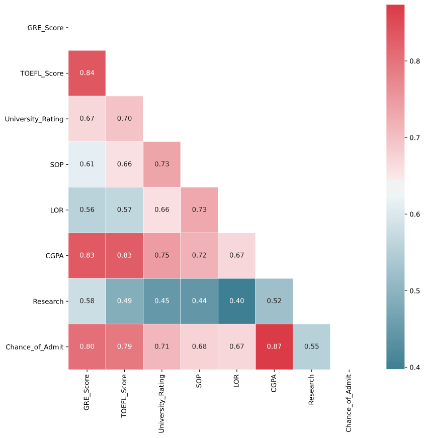

From the above figure, we can see that there are certain variables that are correlated with one another.

• CGPA and GRE score (r = 0.80)
• CGPA and TOEFL score (r = 0.83)
• University rating and TOEFL score (r = 0.70)
• SOP and University rating (r = 0.73)
• CGPA and SOP (r = 0.72) and so on.

So, as the rule of thumb, if correlation (r) > 0.4 we need to remove these correlated variables to make the data model ready. Though the decision of keeping a variable entirely depends on the purpose of modelling.

Another approach is eliminating correlated variables by calculating the Variance Inflation Factor (VIF).

Variance Inflation Factor

Multicollinearity occurs when two or more independent variables are highly correlated with one another in a regression model. Multicollinearity can be problematic because, in case of a regression model, we would not be able to distinguish between the individual effects of the independent variables on the dependent variable.

One way of estimating multicollinearity by estimating a Variance Inflation Factor (VIF). VIF score of an independent variable represents how well the variable is explained by other independent variables.

• VIF starts at 1 and has no upper limit
• VIF = 1: indicates no correlation between an independent variable and the other variables
• VIF > 5 or 10: indicates high multicollinearity between an independent variable and the others

Let’s define a VIF computation function calculate_vif( )

def calculate_vif(X):
  vif = pd.DataFrame()
  vif["variables"] = X.columns
  vif["VIF"] = [variance_inflation_factor(X.values, i) for i in  range(X.shape[1])]
  return(vif)

Let’s remove the dependent variable (Chance of admission) and save this to object X. The computation of VIF shows that a majority of the variable has a VIF score > 10.

X = admission.iloc[:,:-1]
calculate_vif(X)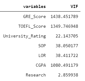

Let’s remove the GRE_Score, TOEFL_Score, Chance_of_Admit, LOR, SOP, University_Rating and check whether the VIF value now withing the permissible limits (<5). After trial and error, I found that keeping CGPA and Research variable in the data set keeps the VIF score below 5.

X = admission.drop(['GRE_Score','TOEFL_Score', 'Chance_of_Admit', 'LOR', "SOP", "University_Rating"], axis=1)

calculate_vif(X)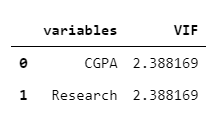

Let’s proceed with the MLR and Logistic regression with CGPA and Research predictors.

Fitting a Multiple Linear Regression Model

Fitting Multiple Linear Regression in Python using statsmodels is very similar to fitting it in R, as statsmodels package also supports formula like syntax.

Here, we are using the R style formula. Chance of Admit predicted by (~) CGPA (continuous data) and Research (binary discrete data). To declare a discrete binary or categorical variable, we need to enclose it under C( ) and you can also set the reference category using the Treatment( ) function. For Research variable I have set the reference category to zero (No research experience: 0).

Once we define the formula, then, we need to use the ordinary least square function using ols( ); where we supply the formula and dataset and fit the model using fit( ) function. The summary of the model estimate is shown below in Figure 9.

formula = "Chance_of_Admit ~ CGPA + C(Research, Treatment(reference = 0))"

mlr = ols(formula, data = admission)

mlr_estimates = mlr.fit()

print(mlr_estimates .summary())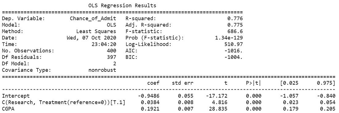

Regression coefficients represent the mean change in the response variable for one unit of change in the predictor variable while holding other predictors in the model constant. From the table estimate, we can observe that the model was fitted using the Least Squares method. Additionally, both estimated coefficients are significant (p<0.05). The CGPA coefficient indicates that for every additional point in CGPA you can expect admission probability to increase by an average of 0.1921. Similarly, a student with research experience is 3.84% more likely to get admission compared to a student with no research experience (reference: 0).

Fitting Binary Logistic Regression Model

The “Binary Logistic Regression” comes under the Binomial family with a logit link function [3]. Binary logistic regression is used for predicting binary classes. For example, in cases where you want to predict yes/no, win/loss, negative/positive, True/False, admission/rejection and so on. There is quite a bit difference exists between training/fitting a model for production and research publication. Here, we will learn how one can model a binary logistic regression and interpret it for publishing in a journal/article.

As the chance of admission is a continuous data thus for demonstration purpose we need to convert it to a binary discrete variable. Here, I assume that if the chance of admission is above 0.7 then a student gets admitted (1) else rejected (0). I make this assumption purely for demonstration purpose.

So, here I have created an “Admission binary” variable that we are going to use as a dependent variable for estimating a binary logistic regression.

The below table shows the Admission_binary variable holds binary values 0 and 1 depending on the dividing criteria (chance of admission).

admission["Admission_binary"] = np.where(admission.Chance_of_Admit > 0.7, 1, 0)

admission.head()

Fitting Binary Logistic Regression

Fitting binary logistic regression is similar to MLR, the only difference is here we are going to use the logit model for model estimation.

Here, we are using the R style formula. Admission_binary predicted by (~) CGPA (continuous data) and Research (binary discrete data). To declare a variable discrete binary or categorical we need to enclose it under C( ) and you can also set the reference category using the Treatment( ) function. For Research variable I have set the reference category to zero (0).

Then, we need to use the logit( ) function where we supply the formula and dataset and fit the model using fit( ) function. The summary of the model estimates is shown in Figure 11.

formula = "Admission_binary ~ CGPA + C(Research, Treatment(reference = 0))"

logit_model = logit(formula, data = admission)

logit_estimates = logit_model.fit()

print(logit_estimates.summary())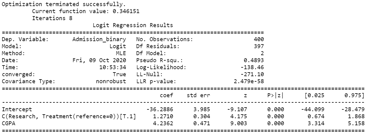

The model is fitted using the Maximum Likelihood Estimation (MLE) method. The pseudo-R-squared value is 0.4893 which is overall good. The Log-Likelihood difference between the null model (intercept model) and the fitted model shows significant improvement (Log-Likelihood ratio test).

The coefficient table showed that Research and CGPA have significant influence (p-values < 0.05; 5% significance level) on admission. The coefficients are positive and in log-odds terms. The interpretation of the model coefficients could be as follows:

Each one-unit increase in CGPA will increase the log odds of admission by 4.2362, and its p-value indicates that it is significant in determining admission. In addition, for Research variable we could say compared to a student with no research, a student with research has 1.2710 log odds of admission holding other variables constant.

Let’s visualize how the probability of admission changes with CGPA values using seaborn’s regression plot (Figure. 12).

sns.regplot(x = "CGPA", y = "Admission_binary", data = admission,
logistic = True, y_jitter = .03)

plt.ylabel("Admission probability")

The interpretation of coefficients in the log-odds term does not make much sense if you need to report it in your article or publication. That is why the concept of odds ratio was introduced.

ODDs Ratio

The ODDS is the ratio of the probability of an event occurring to the event not occurring. When we take a ratio of two such odds it called Odds Ratio.

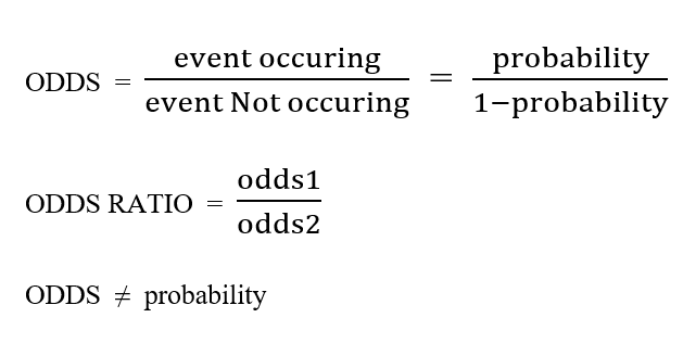
ODDS and ODDS RATIO

Mathematically, one can compute the odds ratio by taking exponent of the estimated coefficients. For example, in the below ODDS ratio table, you can observe that CGPA has an ODDS Ratio of 69.143, which indicates that one unit increase in CGPA increases the odds of admission by 69.143 times. Similarly, the odds of admission is 3.564 times if a student holds some sort of research experience compared to no experience.

round(np.exp(logit_estimates.params), 3)

Even though the interpretation of ODDS ratio is far better than log-odds interpretation, still it is not as intuitive as linear regression coefficients; where one can directly interpret that how much a dependent variable will change if making one unit change in the independent variable, keeping all other variables constant. Thus, to get similar interpretation a new econometric measure often used called Marginal Effects.

Marginal Effects Computation

Marginal effects are an alternative metric that can be used to describe the impact of a predictor on the outcome variable. Marginal effects can be described as the change in outcome as a function of the change in the treatment (or independent variable of interest) holding all other variables in the model constant. In linear regression, the estimated regression coefficients are marginal effects and are more easily interpreted.

There are three types of marginal effects reported by researchers: Marginal Effect at Representative values (MERs), Marginal Effects at Means (MEMs) and Average Marginal Effects at every observed value of x and average across the results (AMEs), (Leeper, 2017) [1]. For categorical variables, the average marginal effects were calculated for every discrete change corresponding to the reference level.

The statsmodels library offers the following Marginal Effects computation:

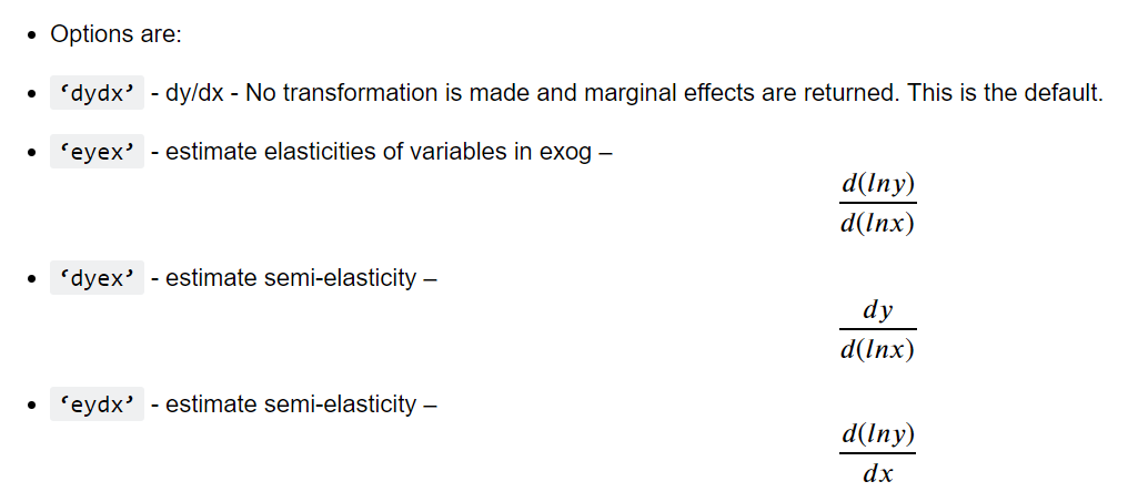
In the STEM research domains, Average Marginal Effects is very popular and often reported by researchers. In our case, we have estimated the Average Marginal Effects (AMEs) of the predictor variables using .get_margeff( ) function and printed the report summary.

AME = logit_estimates.get_margeff(at = "overall", method = "dydx")
print(AME.summary())

The Average Marginal Effets table reports AMEs, standard error, z-values, p-values and 95% confidence intervals. The interpretation of AMEs is similar to linear models. For example, the AME value of CGPA is 0.4663 which can be interpreted as a unit increase in CGPA value increases the probability of admission by 46.63%. Similarly, a student with research experience is 13.99% more likely to get admission compared to no experience.

MLR and binary logistic regression is still a vastly popular ML algorithm (for binary classification) in the STEM research domain. They are still very easy to train and interpret, compared to many sophisticated and complex black-box models.

I hope you learned something new!

Dataset and Code

References

[1] Leeper, T.J., (2017). Interpreting regression results using average marginal effects with R’s margins. Tech. rep.

[2] Mohan S Acharya, Asfia Armaan, Aneeta S Antony: A Comparison of Regression Models for Prediction of Graduate Admissions, IEEE International Conference on Computational Intelligence in Data Science 2019.

[3] Shrikant I. Bangdiwala (2018). Regression: binary logistic, International Journal of Injury Control and Safety Promotion, DOI: 10.1080/17457300.2018.1486503