Introduction

Pearson’s correlation (r) is utilized when we have two numeric variables, and we want to see if there is a linear relationship between those variables. It is often used to eliminate correlated variables before fitting regression models. Similarly, there are few statistical measures of association exists like Cramer’s V and Theil’s U that are used to check association between two nominal variables (categorical variables).

In this blog, we are going to use various libraries to estimate pair-wise Pearson’s correlation matrix, and pair-wise nominal association (using Cramer’s V and Theil’s U).

Further, we will present them using aesthetically beautiful plots (using Matplotlib library).

Article Outline

• Installing libraries
• Loading libraries
• Loading dataset
• Estimating and plotting pairwise Pearson’s Correlation (r) using pandas and matplotlib
• Estimating and plotting pairwise Pearson’s Correlation (r) using dython library
• Estimating Pearson’s correlation (r) using pingouin library (hypothesis testing)
• Estimating and plotting Cramers V (association among nominal variables) using association_metrics library
• Estimating and plotting Cramers V (association among nominal variables) using dython library
• Estimating and plotting Theil’s U (association among nominal variables) using dython library
• Saving plots
• Dataset and codes download link

About datasets

In this blog, we are going to use two datasets. The dataset name and their description are provided as follows:

• Concrete dataset
• Tips dataset

Concrete Dataset

The concrete dataset [1] obtained from the UCI Machine Learning library.

The dataset includes the following variables, which are the ingredients for making durable high strength concrete.

Cement: kg in a m3 mixture
Blast Furnace Slag: kg in a m3 mixture
Fly Ash: kg in a m3 mixture
Water: kg in a m3 mixture
Superplasticizer: kg in a m3 mixture
Coarse Aggregate: kg in a m3 mixture
Fine Aggregate: kg in a m3 mixture
Age: Day (1~365)
Concrete compressive strength: MPa

where m3: meter cube and MPa: Megapascal.

Tips Dataset

The data was reported in a collection of case studies for business statistics. The dataset is also available through the Python library Seaborn [2].

The Tips data contains 244 observations and 7 variables (excluding the index). The variables descriptions are as follows:

bill: Total bill (cost of the meal), including tax, in US dollars
tip: Tip (gratuity) in US dollars
sex: Sex of person paying for the meal (Male, Female)
smoker: Presence of smoker in a party? (No, Yes)
weekday: day of the week (Saturday, Sunday, Thursday and Friday)
time: time of day (Dinner/Lunch)
size: the size of the party

Installing libraries

The first step is to install the following libraries in your python environment.

pip install pandas                # data loading and wrangling
pip install matplotlib            # plots
pip install seaborn               # statistical plots
pip install association_metrics   # correlation/association & plot
pip install dython                # Correlation/association & plot
pip install pingouin              # Hypothesis testing

Importing libraries
Next, import the following libraries.

import numpy as np # for data crunching
import pandas as pd # Data manipulation
import matplotlib.pyplot as plt # Plotting
import seaborn as sns # Statistical plots and tips data

Loading dataset
Let’s read the Concrete dataset using pandas .read_csv( ) method. Print the first five observations using the .head( ) method.

concrete = pd.read_csv("concrete.csv")
concrete.head()

Once the data is loaded, the next step is to check the data information. This is to confirm that all the variables are of numerical type so that we can compute a correlation coefficient (r).

concrete.info()

As per the output, all the variables are numeric type, i.e., either integer or float type.

Estimating Pearson’s Correlation (r) between numerical variables

Parametric Correlation: Pearson correlation (r), is a linear association between two variables and presented in a range of -1 to +1.

Non-parametric Correlation (r): Kendall tau and Spearman rho, are rank-based correlation coefficients (ranges between -1 to +1).

First, we will try the pandas inbuilt corr( ) method on the concrete dataset to compute Pearson’s (r) and round it to two decimal places.

cor_df = concrete.corr(method = "pearson").round(2)
cor_df

It can be noted that few variable pairs are highly correlated. For example, we can see that the correlation between cement and strength is +0.50, similarly water and strength variable pair has a correlation strength of -0.29.

Pearson’s pairwise correlation plot using Pandas and matplotlib library

Once we have the pair-wise correlation matrix, we can generate a plot to illustrate it.

To generate the plot, we need to go through the following steps.

Step 1: Create a figure and axis object with matplotlib’s subplots( ) method.
Step 2: Generate the figure using the ax.imshow( ). Here we have supplied a default Blues colormap and set the minimum (-1) and maximum values (+1).
Step 3: Set the x and y ticks using set method
Step 4: Resize the tick parameters using tick_params( ) method
Step 5: Add a colour-bar using ax.colorbar( ) method to relate the colour gradient to correlation strength
Step 6: Loop through coordinates (x, y) and correlation (r) values using np.ndenumerate( ) method and annotate the values using ax.annotate( ) method.

# Step 1: Initiating a fig and axis object
fig, ax = plt.subplots(figsize = (12, 10))
# Step 2: Create a plot
cax = ax.imshow(cor_df.values, interpolation='nearest', cmap = 'Blues', vmin = -1, vmax = 1)
# Step 3: Set axis tick labels 
ax.set_xticks(ticks = range(len(concrete.columns)),
              labels = concrete.columns)
ax.set_yticks(ticks = range(len(concrete.columns)),
              labels = concrete.columns)
# Step 4: Resize the tick parameters
ax.tick_params(axis = "x", labelsize = 12, labelrotation = 90)
ax.tick_params(axis = "y", labelsize = 12, labelrotation = 0)
# Step 5: Adding a color bar
fig.colorbar(cax).ax.tick_params(labelsize = 12)
# Step 6: Add annotation
for (x, y), t in np.ndenumerate(cor_df):
    ax.annotate("{:.2f}".format(t),
                 xy = (x, y),
                 va = "center", # vertical position
                 ha = "center") # horizontal position

Estimating and Plotting Pearson’s pairwise correlation coefficients using dython library

We can generate the same pairwise correlation plot using dython library, with just two lines of code.

Here, the associations( ) method automatically apply the “Pearson” correlation method on the numerical variables and generates the plot.

# using dython library
from dython.nominal import associations
# Step 1: Instantiate a figure and axis object
fig, ax = plt.subplots(figsize=(16, 8))
# Step 2: Creating a pair-wise correlation plot 
# Saving it into a variable(r)
r = associations(concrete, ax = ax, cmap = "Blues")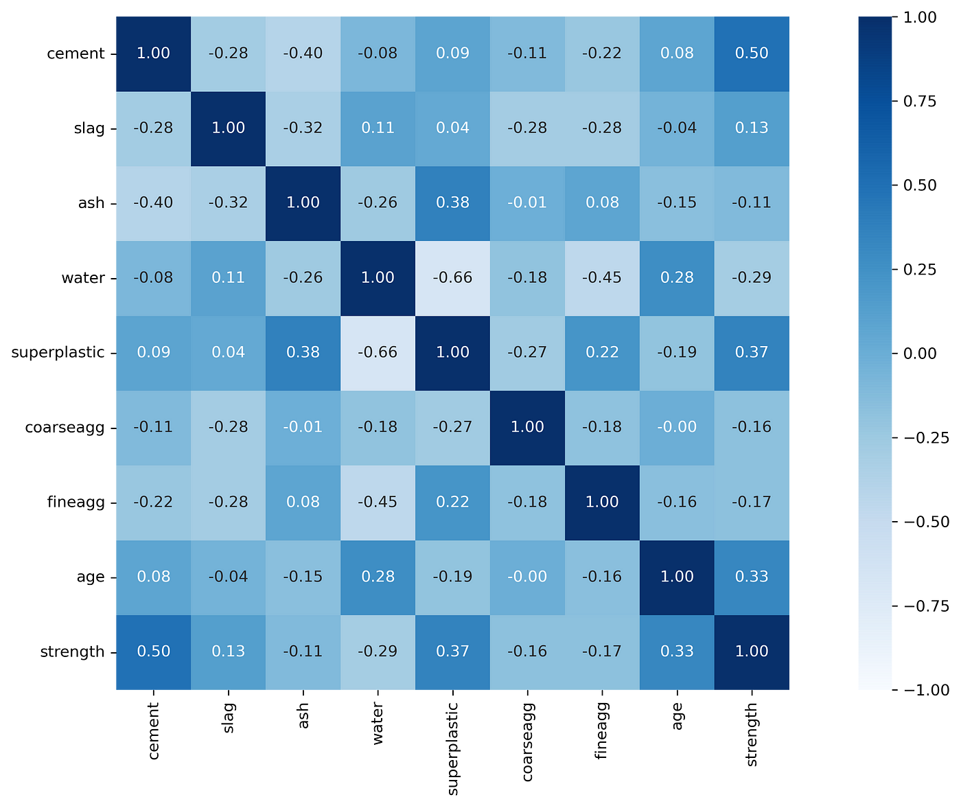

The saved variable contains two objects, i) The correlation matrix and ii) Axis object.

Let’s print the correlation matrix.

r["corr"].round(2)

Estimating Pearson’s correlation using pingouin library

Occasionally, we need to perform a hypothesis test just to report the correlation strength (r) and the p-value.

pingouin library comes in handy which provides different statistics for the pair-wise correlation, including p-value.

Documentation link 1
Documentation link 2

We usually test the following hypothesis while computing correlation.
Null Hypothesis (H0): True correlation is equal to zero.
Alternative Hypothesis (H1): True correlation is not equal to zero.

Here for example, we would like to compute the correlation between four variables which are “cement”, “water”, “strength” and “superplastic”.

# Import library as pg
import pingouin as pg
# Perform a hypothesis testing
(
pg.pairwise_corr(concrete,
        columns = ["cement", "water", "strength", "superplastic"],
        method = 'pearson')
  .round(3)
)

The results show that the probability of all pair-wise correlation values are lower than the conventional 5% (P<0.05), thus here the alternative hypothesis is true.

Estimating Cramer’s V association among nominal variables

In statistics, Cramér’s V (sometimes referred to as Cramér’s phi and denoted as φc) is a measure of association between two nominal variables [3]. The value ranges 0 to 1, where 0 indicates no association and 1 indicates a perfect association.

Cramer’s V facts:

• The value ranges between 0 and 1
• It is a symmetrical association measure [V(x, y) = V(y, x)]

For estimating the Cramer’s V we are going to use the tips dataset.

# Loading tips dataset
tips = sns.load_dataset("tips")
# Print first five observations
tips.head()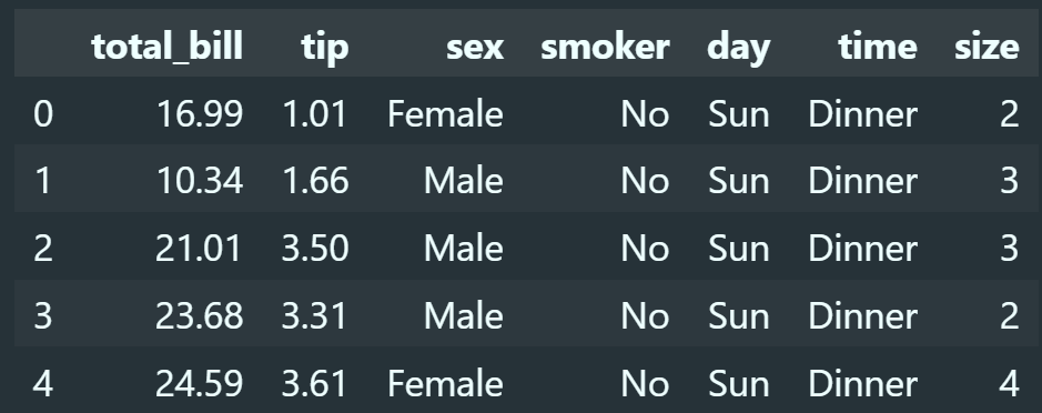

Generating Cramer’s V pairwise matrix plot using `association_metrics` library

To compute the pairwise Cramer’s V association matrix, we need to go through the following steps.

Step 1: import association_metrics as sm.
Step 2: Use a lambda function to convert all object columns to categorical columns.
Step 3: use CramersV( ) method on the dataset.
Step 4: use .fit( ) method to fit the estimator to compute values.

# Using association_metrics library
import association_metrics as am
# Convert object columns to Category columns
df = tips.apply(
        lambda x: x.astype("category") if x.dtype == "O" else x)
# Initialize a CramersV object using the pandas.DataFrame (df)
cramers_v = am.CramersV(df)
# It will return a pairwise matrix filled with Cramer's V, where 
# columns and index are the categorical variables of the passed     # pandas.DataFrame
cfit = cramers_v.fit().round(2)
cfit

The next step is to generate a pair-wise association plot, the same way we did it for Pearson’s correlation coefficient (r).

# Instantiating a figure and axes object
fig, ax = plt.subplots(figsize = (10, 6))
# Generate a plot
cax = ax.imshow(cfit.values, interpolation='nearest', cmap='Blues', vmin=0, vmax=1)
# Setting the axes labels
ax.set_xticks(ticks = range(len(cfit.columns)),
              labels = cfit.columns)
ax.set_yticks(ticks = range(len(cfit.columns)),
              labels = cfit.columns)
# Setting tick parameters
ax.tick_params(axis = "x", labelsize = 12, labelrotation = 0)
ax.tick_params(axis = "y", labelsize = 12, labelrotation = 0)
# Adding a colorbar
fig.colorbar(cax).ax.tick_params(labelsize = 12)
# Adding annotations
for (x, y), t in np.ndenumerate(cfit):
    ax.annotate("{:.2f}".format(t),
                xy = (x, y),
                va = "center",
                ha = "center").set(color = "black", size = 12)

Generating Cramer’s V pairwise association plot using dython library

The same pair-wise association plot can be generated using dython library using two lines of codes. Just, we need to provide categorical columns (object) and nom_nom_assoc = ‘cramer’.

Note:
[1] For dython library, we must supply the categorical columns as “object” type. Here, we converted “categorical” columns to “object” columns.
[2] By default, dython library enables Cramer’s V bias correction (cramers_v_bias_correction=True); thus values estimated using dython library will be slightly different from association_metrics library.

# Importing library
from dython.nominal import associations
# Convert categorical columns to object columns
df = tips.apply(
        lambda x: x.astype("object") if x.dtype == "category" else x)
# Instantiate a figure and axis object
fig, ax = plt.subplots(figsize = (12, 7))
# Estimate and generate Cramer's V association plot
cramers_v = associations(df[["sex", "smoker", "day", "time"]],
             nom_nom_assoc = 'cramer',
             ax = ax,
             cmap = "Blues")

The saved object cramers_v contains two sub-objects, i) the pair-wise association value matrix and ii) axis object.

Let’s print the association matrix and round up to two decimal places.

cramers_v["corr"].round(2)

Let’s access the axis object that we can later use for plot modifications.

Note: This method of axis object retrieval is appropriate only when if we have not instantiated the figure and axis objects using Matplotlib’s .subplots( ).

cramers_v["ax"]

<AxesSubplot:>

Generating Theil’s U pairwise association plot using dython library

In statistics, Theil’s U is a measure of association between two nominal variables [4, 5]. Similar to Cramer’s V, the value ranges 0 to 1, where 0 indicates no association and 1 indicates a perfect association.

Theil’s U facts:

• The value ranges between 0 and 1
• It is an asymmetrical association measure [U(x, y) ≠ U(y, x)]

Here, we are going to use the dython library and will supply nom_nom_assoc = ‘theil’.

Note: for dython library, we must supply the categorical columns as “object” type. Here, we converted “categorical” columns to “object” columns.

# Loading libarary
from dython.nominal import associations
# Convert categorical columns to object columns
df = tips.apply(lambda x: x.astype("object") if x.dtype == "category" else x)
# Instantiate a figure and axis object
fig, ax = plt.subplots(figsize = (10, 7))
# Estimate and generate Theil's U association plot
theils_u = associations(df[["sex", "smoker", "day", "time"]],
             nom_nom_assoc = 'theil',
             ax = ax,
             cmap = "Blues")

Same way, we can retrieve the association matrix.

theils_u["corr"].round(2)

Let’s retrieve the axis object.

theils_u["ax"]

<AxesSubplot:>

Saving Plots

We have instantiated the figure (fig) object for each of the plots generated above. Thus, after generating a particular plot, we can save the plot using .savefig( ) method.

# bbox_inches = "tight" removes unnecessary borders
# You can change the "dpi" value to get a higher resolution plot
fig.savefig("figurename.png", dpi = 300, bbox_inches = "tight")

These are the various ways to generate aesthetically beautiful publication ready correlation and association plots.

Click here for the data and code

References

[1] I-Cheng Yeh, “Modeling of the strength of high-performance concrete using artificial neural networks,” Cement and Concrete Research, Vol. 28, №12, pp. 1797–1808 (1998).

[2] Bryant, P. G. and Smith, M. A. (1995), Practical Data Analysis: Case Studies in Business Statistics, Richard D. Irwin Publishing, Homewood, IL.

[3] Cramér, H., 2016. Mathematical methods of statistics, in: Mathematical Methods of Statistics (PMS-9), Volume 9. Princeton University press, pp.
1–575.

[4] Theil, H., 1958. Economic policy and forecasts.

[5] Theil, H., 1966. Applied economic forecasting, rand mcnally and company.

I hope you learned something new!