Rahul Raoniar
- posted on
- Comments Off on Start Your CNN Journey with PyTorch in Python

Learn how to Classify Hand Written Digits using a Convolutional Neural Network (CNN).
Article Outline
- Introduction
- About PyTorch
- Neural Network’s Data Representation Learning Process
- About MNIST Dataset
- MNIST Data Loading
- Setting the Model Configuration using Sequential module
- Setting Loss Criteria and Optimizer
- Model Training and Performance Evaluation
- Plotting Training Loss and Test Accuracy
- CNN Tutorial Code
Introduction
The world of Machine learning is fascinating. Nowadays ML is everywhere. If you are learning data science and have a grasp on fundamental ML tools such as regression and classification then you will be eagerly waiting to learn about more complex ML tools, such as Neural Networks. Neural networks are fascinating, not just because of its name but how it learns complex data representations that sometimes impossible for even human beings. Let’s start with a simple example “recognizing handwritten digits”. Recognizing a digit is a very simple process for humans but very complex for machines. Let’s see how the computer learns different digits.
This article gives you an overview of how to use PyTorch for image classification. Here, we will be discussing step by step process involved in developing a convolutional neural network that accurately recognizes handwritten digit.
About PyTorch
Let’s first get familiar with PyTorch. PyTorch is a python based ML library based on Torch library which uses the power of graphics processing units. This library is developed by Facebook’s AI Research lab which released for the public in 2016. Though google’s TensorFlow is already available in the market, the arrival of PyTorch has given tough competition.
The PyTorch library is currently immensely popular among ML practitioners and developers. Its popularity is mainly being driven by a smoother learning curve and a cleaner interface, which is providing developers with a more intuitive approach to build neural networks.
After learning TensorFlow when I started learning PyTorch, I was really amazed by the OOP based coding style, which is more pythonic, and it the best way to learn a neural network’s architecture and functionality. In one word, I could say PyTorch is awesome. Just give it a try.
Neural Network’s Data Representation Learning Process
Learning how a neural network works would require some time investment, but one can learn it with a little bit of dedication. If you know how it works then good, if not then you could go first for the following resources.
If you like video tutorials, just go for tutorials of “Andrew Ng” YouTube Link or if you are a reader go for this blog: Neural Network
Once you understand how it works this will give you the power of wand…just like Harry Potter. Well, let’s talk about how this wand (NN) works.
The neural network learns data representation using the following five steps:
- Random weights initialization
2. Passing the weighted sum (sum of input * weights) through an activation function and calculating the output
3. Calculating the loss (the difference between the actual output and predicted)
4. Computing the gradients through the backpropagation
5. Updating the weights with better ones
The 1 to 3 steps called forward pass and 4, 5, called a backward pass. The whole process (one forward pass followed by a backward pass) called an epoch, where the whole dataset goes through this forwards and backward pass once. This process goes multiple times to identify the most exact set of weights (data representation) that predicts the outputs most accurately.
For more complex operations such as classification of images instead of simple neural networks, an advanced version of the neural network is used called Convolutional Neural Networks (CNN). ConvNets or CNNs is one of the main modeling techniques used to perform image recognition, image classification, object detection, and face recognition. Because of its convolutional strategy (feature extraction), it able to identify the important data representation from different images, which makes it more powerful than normal deep networks.
To learn how this works, you might go for the following resources:
Andrew Ng’s CNN tutorials on YouTube: Convolutional Neural Network
Blogs: CNN blog1, CNN blog2, CNN blog3, CNN blog4, CNN blog5
About MNIST Dataset
MNIST (“Modified National Institute of Standards and Technology”) is the de facto “Hello World” dataset of computer vision. Since its release in 1999, this classic dataset of handwritten images has served as the basis for benchmarking classification algorithms. The MNIST dataset of handwritten digits has a training set of 60,000 examples (digits: 0 to 9)and a test set of 10,000 examples. It is a subset of a larger set available from NIST. The dataset is used as the basis for learning and practicing how to develop, evaluate, and use different machine learning algorithms for image classification from scratch. Even kaggle.com has organized a competition “Digits Recognizer” where more than 2000 teams competed to build the most accurate classifier. More details about the dataset, including algorithms that have been tried on it and their levels of success, can be found at http://yann.lecun.com/exdb/mnist/index.html

Importing relevant libraries
The first step is to install the PyTorch library and load relevant modules/classes. For more information on how to install Pytorch click the link.
# Importing relevant libraries
import torch
import torchvision
import torchvision.transforms as transforms
import torch.optim as optim
import torch.nn as nn
MNIST Data Loading
It takes very few steps to load data in PyTorch. But if you are new to PyTorch, it is recommended to start with a cleaned and preprocessed data set. Pytorch has an inbuilt function that helps you to download the cleaned and preprocessed data set for learning purposes.
A) Data Transformation
First, we need to define a transformer before feeding the data into the modeling pipeline. Initially, we will use torchvision.transforms class to convert the dataset.
1. transforms.ToTensor(): transform the dataset into PyTorch Tensor
2. transforms.Normalize(): normalize pixel values.
In machine learning, data normalization before model training is a very common adapted approach. Normalizing apply the following for each channel: image = (image - mean) / std
In our casemean, std are passed as 0.5, 0.5. This will normalize the image and bring it to in the range of -1 and +1. In other words, the value 0 will be converted to (0-0.5)/0.5 = -1, the maximum value of 1 will be converted to (1-0.5)/0.5 = 1. As our data is in grayscale that’s why we only applied 0.5 once; for RGB channel it will be transformed.Normalize((0.5, 0.5, 0.5), (0.5, 0.5, 0.5))
# Transforming to torch tensors and normalizing
transform = transforms.Compose([transforms.ToTensor(),
                               transforms.Normalize(
                                 (0.5, ), (0.5, ))])
B) Data Loading
The next step is to prepare the train and test data set. We can download it by setting the argument download = True. For train data, we set the train argument to True and for applying transformation we set transform = transform.
# Preparing training and testing dataset
trainset = torchvision.datasets.MNIST('mnist', train=True,
                                      download=True,
                                      transform=transform)
testset = torchvision.datasets.MNIST('mnist', train = False,
                                     download=True,
                                     transform=transform)
C) Preparing Data Loader
The next step is to prepare a train and test loader. We further set the argument batch_size = 100, so that during training this will fetch the data in batches of 100. For the train loader, we set the argument shuffle = True so that during training the data sequence bias can be removed and the training becomes more generalized. We set the number of workers (num_workers = 0) i.e. the number of PC cores to use. For the larger dataset, one can set it to the required value.
# Prepare train and test loader
train_loader = torch.utils.data.DataLoader(trainset,
                                           batch_size = 100,
                                           shuffle = True,
                                           num_workers=0)
test_loader = torch.utils.data.DataLoader(testset,
                                          batch_size = 100,
                                          shuffle = False,
                                          num_workers=0)
Observing the first 40 digits
Before jumping into the training process, let’s go for some basic exploratory analysis. Let’s visualize the first 40 training images.
# Observing first 40 images
figure = plt.figure()
num_of_images = 40
for index in range(1, num_of_images + 1):
    plt.subplot(4, 10, index)
    plt.axis('off')
    plt.imshow(trainset.data[index],
cmap='gray_r')Data Inspection
The training and testing data shapes showed that the training data has 60,000 examples of 28 x 28 pixels. Similarly, the test set includes 10,000 examples with the same size.
print(trainset.data.shape)
print(testset.data.shape)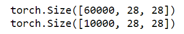
The train loader shape revealed that there are 100 images in each batch and each image has 28 x 28 pixels, and 100 images have 100 labels, which is absolutely correct.
data_iter = iter(train_loader)
images, labels = data_iter.next()
print(images.shape)
print(labels.shape)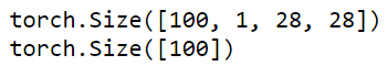
Setting the Model Configuration using Sequential module — init method
There is two way we can define the neural network’s style layout. One is using the functional module and another is using the sequential module. Though there is no performance difference, the later is easy to implement.
We will go for the sequential method. In the model definition, we have to provide two layers, one for feature extraction and another for classification.
- features extraction layer definition
The feature layers definition actually extracts the image features layer by layer. Here we have used four convolutional layers. Additionally, two max pool (MaxPool2d) layers after every second convolutional layer and three batch normalization (BatchNorm2d) layers are applied. For non-linear transformation, we used the Relu activation function.
nn.Conv2d:
nn.Conv2d(in_channels=1,
          out_channels=5,
          kernel_size=3,
          stride=1,
padding=1)- in_channels (int) — Number of channels in the input image (for grayscale image: 1 and for RGB image: 3)
- out_channels (int) — Number of channels produced by the convolution. Here we have defined 5, 10, 20, 40. The output of every out_channes will be the input (in_channels) for the next convolutional layer.
- kernel_size (int or tuple) — Size of the convolving kernel. Here, we have chosen 3.
- stride (int or tuple, optional) — Stride of the convolution. (Default: 1)
- padding (int or tuple, optional) — Zero-padding added to both sides of the input (Default: 0). Here, we have selected padding = 1.
- Here, we have used a Relu() activation function for applying nonlinearity.
nn.MaxPool2d(2, 2)
- Each pooling layer i.e., nn.MaxPool2d(2, 2) halves both the height and the width of the image, so by using 2 pooling layers, the height and width are 1/4 of the original sizes.
nn.BatchNorm2d( )
Batch-normalization makes the training of convolutional neural networks more efficient, while at the same time having regularization effects.
2. classification layer definition
We pass the extracted features, in the sequential classification layer. In the feature extraction layers, 2 max-pooling layers, halves both the height and the width of the image that why we get the 7 x 7 (28/4) size with the last output of the out_channels 40. We pass them to the sequential layer. Here we used hidden layers of size 200 and 500 neurons.
Dropout: Dropout is an effective technique to avoid overfitting [1]. Typically, dropout is applied in fully-connected neural networks. Here, we have applied it after the first hidden layer in the classification layer. In the Dropout(p = 0.5), p = 0.5 indicates the probability at which outputs of the layer are dropped out.

# Declare all the layers for classification
        self.classifier = nn.Sequential(
            nn.Linear(7 * 7 * 40, 200),
            nn.ReLU(inplace=True),
            nn.Dropout(p=0.5),
            nn.Linear(200, 500),
            nn.ReLU(inplace=True),
            nn.Linear(500, 10))
Next, we need to define the forward method. Here, we pass the data into the sequential features layer to extract the image features. Then we squeeze the features into one dimension using x.view( ) and pass to the classifier layer.
def forward(self, x):

        # Apply the feature extractor in the input
        x = self.features(x)

        # Squeeze the three spatial dimensions in one
        x = x.view(-1, 7 * 7 * 40)

        # Classify the images
        x = self.classifier(x)
        return x
Here is the sequential blueprint of the overall CNN model.
class Net(nn.Module):
    def __init__(self):
        super(Net, self).__init__()

        # Declare all the layers for feature extraction
        self.features = nn.Sequential(nn.Conv2d(in_channels=1,
                                                out_channels=5,
                                                kernel_size=3,
                                                stride=1,
                                                padding=1),
                                      nn.ReLU(inplace=True),
                                      nn.Conv2d(in_channels=5,
                                                out_channels=10,
                                                kernel_size=3,
                                                stride=1,
                                                padding=1),
                                      nn.MaxPool2d(2, 2),
                                      nn.ReLU(inplace=True),
                                      nn.BatchNorm2d(10),
                                      nn.Conv2d(in_channels=10,
                                                out_channels=20,
                                                kernel_size=3,
                                                stride=1,
                                                padding=1),
                                      nn.ReLU(inplace=True),
                                      nn.BatchNorm2d(20),
                                      nn.Conv2d(in_channels=20,
                                                out_channels=40,
                                                kernel_size=3,
                                                stride=1,
                                                padding=1),
                                      nn.MaxPool2d(2, 2),
                                      nn.ReLU(inplace=True),
                                      nn.BatchNorm2d(40))

        # Declare all the layers for classification
        self.classifier = nn.Sequential(
            nn.Linear(7 * 7 * 40, 200),
            nn.ReLU(inplace=True),
            nn.Dropout(p=0.5),
            nn.Linear(200, 500),
            nn.ReLU(inplace=True),
            nn.Linear(500, 10))

    def forward(self, x):

        # Apply the feature extractor in the input
        x = self.features(x)

        # Squeeze the three spatial dimensions in one
        x = x.view(-1, 7 * 7 * 40)

        # Classify the images
        x = self.classifier(x)
        return x
Setting Loss Criteria and Optimizer
For backpropagation, we need to set a loss estimator and an optimizer. We first instantiated the Net( ) and saved under the model object. Next, we defined the loss criteria. As this is a multiclass classification (0 to 9) thus, we used CrossEntropyLoss( ). Additionally, we also defined an optimizer. Here, we have selected the Adaptive Moment (Adam) optimizer with learning rate = 3e-4 and a weight decay = 0.001 ((l2 regularization). The l2 regularization simply penalizes large weights and improves the network’s performance.
# Instantiate the network
model = Net()
# Instantiate the cross-entropy loss
criterion = nn.CrossEntropyLoss()
# Instantiate the Adam optimizer
optimizer = optim.Adam(model.parameters(),
                       lr = 3e-4,
                       weight_decay= 0.001)
Calculating iterations and epochs
- epoch: 1 epoch means training all samples one time.
- In our training example, we have 60000 examples to train and we selected a batch_size of 100. So, for one epoch we need (60000/100) = 600 iterations. I have trained this model several times and found that in 10 epochs (approx.) the CNN reaches 99% (approx.) test accuracy.
- So, to achieve 10 epochs, the total iteration is required 10*600 = 6000
- Here, we will train the model for 10 epochs
# batch_size, epoch and iteration
batch_size = 100
features_train = trainset.data.shape[0]
n_iters = 6000
num_epochs = n_iters/(features_train/batch_size)
num_epochs = int(num_epochs)
print("number of epochs: " + num_epochs)
number of epochs: 10
Model Training and Performance Evaluation
- Model Training Steps
The model training includes the following steps:
Step 1: iterating over train_loader to obtain train images and labels
for i, data in enumerate(train_loader, 0):
        train, labels = data
Step 2: Setting the initial gradients to zero so that it will clear any weight stored from previous training. This is just for a fresh start.
# Clear gradients
        optimizer.zero_grad()
Step 3: Computing the model output
# Forward propagation
        outputs = model(train)
Step 4: Compute the loss, from the difference between the actual and predicted outputs
# Calculate relu and cross entropy loss
        loss = criterion(outputs, labels)
Step 5: Calculating the gradient using the estimated loss
# Calculating gradients
        loss.backward()
Step 6: Updating the weights
# Update weights
        optimizer.step()
2. Model Evaluation Steps
The model evaluation is done on the remaining test dataset (10,000 samples). The model evaluation involves the following steps:
Step 1: iterating over the test_loader to obtain test images and labels
for i, data in enumerate(test_loader, 0):
                test, labels = data
Step 2: Calculating the outputs and predicted classes using the torch.max( )
# Forward propagation
                outputs = model(test)

                # Get predictions from the maximum value
                predicted = torch.max(outputs.data, 1)[1]
Step 3: Calculating the prediction accuracy on the test dataset.
# Total number of labels
                total += len(labels)

                correct += (predicted == labels).sum()

            accuracy = 100 * correct / float(total)
Here, we have set a counter that counts the iteration. After every 50 counts (cumulative), this calculates the training loss, test accuracy, and iteration count, and store inside loss_list, accuracy_list and, iteration_list so that we could use it for visual inspection (plotting).
loss_list = []
iteration_list = []
accuracy_list = []
additionally, we printed the training loss and test accuracy at every 600 iterations (1 epoch) to observe how the CNN model is performing. We trained the model for 6000 iterations (10 epochs).
if count % 600 == 0:
            # Print Loss
            print('Iteration: {}  Loss: {}  Accuracy: {} %'.format(count, loss.data, accuracy))
Here is the blueprint of the overall model training and testing.
# CNN model training
count = 0
loss_list = []
iteration_list = []
accuracy_list = []
for epoch in range(num_epochs):
    for i, data in enumerate(train_loader, 0):
        train, labels = data

        # Clear gradients
        optimizer.zero_grad()

        # Forward propagation
        outputs = model(train)

        # Calculate relu and cross entropy loss
        loss = criterion(outputs, labels)

        # Calculating gradients
        loss.backward()

        # Update weights
        optimizer.step()

        count += 1

        if count % 50 == 0:
            # Calculate Accuracy
            correct = 0
            total = 0
            # Iterate through test dataset
            for i, data in enumerate(test_loader, 0):
                test, labels = data

                # Forward propagation
                outputs = model(test)

                # Get predictions from the maximum value
                predicted = torch.max(outputs.data, 1)[1]

                # Total number of labels
                total += len(labels)

                correct += (predicted == labels).sum()

            accuracy = 100 * correct / float(total)

            # store loss value and iteration
            loss_list.append(loss.data)
            iteration_list.append(count)
            accuracy_list.append(accuracy)
        if count % 600 == 0:
            # Print Loss
            print('Iteration: {}  Loss: {}  Accuracy: {} %'.format(count, loss.data, accuracy))
The CNN Model evaluation on the test dataset showed that with 10 epochs our CNN model achieved up to 99% (approx) classification accuracy on the test dataset. This showed the power of modern ML algorithms, but this comes at a cost; such as it requires huge training examples and high computational power. In the kaggle.com “Digits Recognizer” competition, the winner has achieved an accuracy of 99.7%, which is astonishing. The competitor used image augmentation techniques available in the TensorFlow library to generate 25 million images that lead him to the top of the leader board. You can also try this approach and see whether this would work with PyTorch.
Plotting Training Loss and Test Accuracy
Let’s visualize the training loss and testing accuracy over the iteration space using matplotlib’s pyplot class.
import matplotlib.pyplot as plt
# visualization of training loss
plt.plot(iteration_list,loss_list)
plt.xlabel("Number of iteration")
plt.ylabel("Loss")
plt.title("CNN: Loss vs Number of iteration")
plt.show()
# visualization of test accuracy
plt.plot(iteration_list,accuracy_list,color = "red")
plt.xlabel("Number of iteration")
plt.ylabel("Accuracy")
plt.title("CNN: Accuracy vs Number of iteration")
plt.show()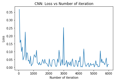
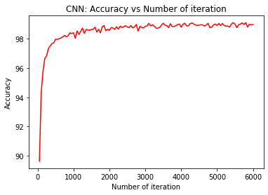
From the above plots, we can observe that after 3000 iterations (5 epochs) there are only small improvements in the model performance. Hence, we can use early stopping criteria to stop training after certain iterations, to reduce the model overfitting.
Now, you are familiar with the hello world of CNN. I hope you learned something new from this blog.
I would like to thank dataiteam for their wonderful kernel on Kaggle’s Digits Recognizer challenge, which helped and motivated me to learn and write this PyTorch blog.
References
[1] Srivastava, N., Hinton, G., Krizhevsky, A., Sutskever, I. and Salakhutdinov, R., 2014. Dropout: a simple way to prevent neural networks from overfitting. The journal of machine learning research, 15(1), pp.1929–1958.
Blog Image Credit
Photo by Markus Winkler on Unsplash