Data Manipulation in Python using the dfply Package (dplyr-Style)

Introduction

I have been working with R programming language since 2018. R is a statistical programming language very popular among data science enthusiasts, statisticians, and academicians. If you have ever used R then you might have encountered the popular data manipulation package called “dplyr” developed by [Hadley Wickham [aut, cre], Romain François [aut], Lionel Henry [aut], Kirill Müller [aut] and RStudio [cph, fnd] ]. This package contains several essential tools that make your data manipulation fast, fluent, and fun. The dplyr library/package allows you to write functions in chained order, which is very very helpful.

I personally use R for data manipulation and Python for ML. Even before starting a model training in Python I usually perform some sort of manipulation to better understanding the dataset. In the Python world, the Pandas package is one of the most popular packages usually used for data manipulation but I personally like the chaining style of the dplyr package when I need to perform very complex operations.

You can enjoy the fun of the dplyr package in Python too. Kiefer Katovich has implemented similar essential functions of dplyr into a new Python package known as dfply. The dfply package’s philosophy is primarily based on the following major functions and it is constantly updated by the package maintainer.

• select() picks variables based on their names.
• filter_by() picks cases based on their values.
• mutate() adds new variables that are functions of existing variables
• summarise() reduces multiple values down to a single summary.
• arrange() changes the ordering of the rows.

The current article focuses on showing the core dfply functionality using the popular hflights dataset/pandas data frame.

Article Outline

• Introduction
• dfply installation
• Description of hflights dataset
• Data Manipulation using primary dfply functions
• Others important functions
• Dataset and code link

dfply installation

The very first step is to install the dfply package using pip or anaconda installation. This package requires Python 3.

# pip installation
pip install dfply
# conda installation
conda install -c tallic dfply

Description of hflights dataset

The hflights dataset contains all flights departing from Houston airports IAH (George Bush Intercontinental) and HOU (Houston Hobby). The data set contains the following features/variables.

Year, Month, Day, date of departure, Day of the week of departure (DayOfWeek), Departure and arrival times (DepTime, ArrTime), Unique abbreviation for a carrier (UniqueCarrier), Flight number (FlightNum), Airplane tail number (TailNum), Elapsed time of flight in minutes (ActualElapsedTime), Flight time in minutes (AirTime), Arrival and Departure delays in minutes (ArrDelay, DepDelay), Origin and Destination airport codes (Origin, Dest), Distance of flight in miles (Distance), Taxi in and Out times in minutes (TaxiIn, TaxiOut), Cancelled indicator: 1 = Yes, 0 = No (Cancelled), Diverted indicator: 1 = Yes, 0 = No (Diverted).

Importing essential packages

The first step is to import the essential packages before dive into data manipulation fun.

import pandas as pdfrom dfply import *

Loading hflights dataset

Let’s import the hflights data into the python environment using pandas pd.read_csv() function. I have cleaned the dataset by removing missing values and few columns.

hflights = pd.read_csv("hflights_cleaned.csv", index_col=0)
hflights.head()

Checking the column names

Let’s check the column names using .columns method.

hflights.columns

Introduction to the pipe method of dfply

R’s magrittr package first introduced the pipe operator >>. The operator pipe their left-hand side values forward into expressions that appear on the right-hand side, i.e. one can replace f(x) with x >> f(), where >> is the (main) pipe-operator.

dfply works directly on pandas DataFrames, chaining operations on the data with the >> operator, or alternatively starting with >>= for inplace operations.

Lets Start piping

Observing the head or tail of the data frame

Let’s start with the most common operation observing first or last few row examples using head( ) or tail( ) function but more like dfply way (chaining/piping). Let’s check first 2 rows of hflight data frame by chaining head( ) function with >>.

hflights >> head(2)

Similarly, you can check the last observations/rows to get a glimpse of the data using the tail() function.

A) Selecting and dropping columns

You often need to work with datasets that include a large number of columns/variables but only a few of them will be the variable of interest. Let’s say you want to select Year, Origin, and Dest from hflights dataset and print top 2 rows. The variable selection can be done using X dot -> [X.dot] or quotation ‘var1’ , ‘var2’ … or column index number.

A1) X dot way:

(hflights 
  >> select(X.Year, X.Origin, X.Dest) 
  >> head(2))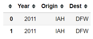

A2) Quote and index-based selection

(hflights >>
 select(0, ['Origin', 'Dest']) >>
 head(2))

A3) starts_with( ):

Sometimes we need to select variables that start with a common name/string/characters. One example could be column names starts with “date” prefix. Here in this dataset, say we want to select columns that start with Arr character.

(hflights >>
 select(starts_with("Arr")) >>
 head(2))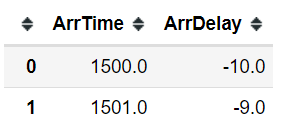

A4. Drop using a tilde (~):

we can put a tilde sign in front of variables to exclude them from the column selection.

Arr_not_in_data = hflights >> select(~starts_with("Arr"))
Arr_not_in_data.columns

The above data frame now doesn’t include columns that start with Arr characters.

A5) columns_from( ): Dropping column UniqueCarrier onwards

The drop function is opposite to selection. We could use the columns_from selection filter along with drop( ) function to drop all columns “UniqueCarrier” onwards and select the top 2 rows of the rest.

(hflights >>
drop(columns_from(X.UniqueCarrier)) >>
head(2))

A6) Column_to() and column_from() together

Let’s say we want to select the first two columns, the last three columns, and the “DayOfWeek” column together. The inclusive = True argument keeps the column with index 1.

(hflights >> 
select(columns_to(1, inclusive=True),
       'DayOfWeek',
       columns_from(-3)) >>
head(2))

B) Subset selection based on filter_by( )

filter_by( ) function helps you to select a subset of a pandas data frame based on logical conditions. Let’s say we want to select a subset of rows where Arrival Delay ≥ 500 and based on this condition we want to select all columns that start with Arr. You can set multiple conditions separated with commas.

(hflights >>
 filter_by(X.ArrDelay >= 500) >>
 select(contains("Arr")) >>
 head(3))

Pulling out columns using pull() function

In case you only care about one particular column at the end of your pipeline, you can pull out a column and returns it as a pandas series. Let’s pull out the ArrTime column based on the condition of ArrDelay≥500

(hflights >>
 filter_by(X.ArrDelay >= 500) >>
 pull('ArrTime') >>
 head(4))

C) Creating new columns using mutate( )

Let’s say we want to calculate the total delay of each flight. This can be calculated using X.ArrDelay + X.DepDelay. We can pass this inside the mutate function and assign to a new column name Total_Delay.

C1) mutate( ):

(hflights >> 
  select(X.ArrDelay, X.DepDelay) >> 
  mutate(Total_Delay = X.ArrDelay + X.DepDelay) >> 
  head(3))

C2) transmute( ):

Sometimes we want the newly generated column data only; to perform different statistical analysis on that. Plotting a histogram could be a great example. In such cases, we could use the transmute( ) function.

(hflights >> 
  select(X.ArrDelay, X.DepDelay) >> 
  transmute(Total_Delay = X.ArrDelay + X.DepDelay) >> 
  head(3))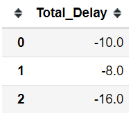

D) sorting rows with arrange( )

Let’s, for example, we want to arrange our dataset based on decreasing values of ArrDelay column. To achieve this we could use the arrange( ) function and supply the ArrDelay column and set the ascending = False.

(hflights >>
 arrange(X.ArrDelay, ascending=False) >>
 select(X.ArrDelay)>>
 head())

E) Summarizing data using summarize( )

Summarize help in computing single row statistics such as mean, standard deviation, minimum and maximum etc.

E1. summarize( ):

For example, if we want to calculate the mean arrival delay and mean departure delay we could you the summarize( ) function and supply the columns with a dot method; in our case mean( ).

(hflights >>
 summarize(mean_arr_delay = X.ArrDelay.mean(),
           mean_dep_delay = X.DepDelay.std()))

E2. summarize_each( ):

In some situation, we need to compute multiple statistics for multiple variables. In such scenarios we could use summarize_each( ) function. Here, in the following example, we applied the mean (np.mean) and standard deviation (np.std) function on ArrDelay and DepDelay.

(hflights >>
 summarize_each([np.mean, np.std], X.ArrDelay, X.DepDelay))

E3. Grouping data using group_by( )

group_by( ) function allows you to group data based on one or multiple columns. This helps us to compute statistics on each group of data separately.

For example, we want to compute the monthly mean and standard deviation of Arrival Delay and Departure Delay. This can be achieved using the group_by(X.Month). We assigned the resulting data frame to monthly_stats variable and printed the first 4 months.

monthly_stats = (hflights >> 
  select(X.ArrDelay, X.DepDelay, X.Month) >> 
  group_by(X.Month) >> 
  summarise_each([np.mean, np.std], X.ArrDelay, X.DepDelay))
monthly_stats.head(4)

E4. Plotting resulting data frame combining pandas plot( )

Instead of getting just only the data frame, we could add a pandas plot function in the resulting data frame. Here, we plotted a line plot using Month on the x-axis and mean Arrival Delay on the y-axis.

(hflights >> 
  select(X.ArrDelay, X.DepDelay, X.Month) >> 
  group_by(X.Month) >> 
  summarise_each([np.mean, np.std],
                 X.ArrDelay,
                 X.DepDelay)).plot(x = "Month",
                                   y = "ArrDelay_mean",
                                   kind = "line")

F) Others important functions

There are plenty of useful functions available in dfply package. Here are a few of them.

F1. Sampling

Taking a random sample in the data science domain is a very common task. A random sample can be obtained supplying fraction argument (frac) or number (n) inside the sample( ) function.

In this example, we used the sample( ) function and supplied fraction (frac) argument. One can also set the replacement to True/False.

hflights >> sample(frac=0.2, replace=False)

if you know how many random samples do you want in advance then use n (number of the sample) argument instead of frac (fraction). Here we set replacement to True.

hflights >> sample(n=4, replace=True)

F2. distinct( ):

The distinct( ) function helps in identifying the number of distinct levels available in a categorical column.

hflights >> distinct(X.Origin) >> select(X.Origin)

F3. rename( ):

The rename() function will rename columns provided as values to what you set as the keys in the keyword arguments.

hflights = hflights >> rename(Destination = X.Dest)
hflights.columns

F4. Count using n( )

Let’s estimate the monthly flights count where Departure Delay ≤ 10 minutes using n( ) function.

(hflights >>
 filter_by(X.DepDelay <= 10) >>
 group_by(X.Month) >>
 summarize(count = n(X.FlightNum)))

F5. mutate( ) + between( )

One can use between( ) function inside the mutate( ) function to create a boolean variable. Here, we have created an arr_delay_btwn boolean variable and coded levels as True if ArrDelay within 1 and 5 else False.

(hflights >> 
 select(X.ArrDelay) >> 
 mutate(arr_delay_btwn = between(X.ArrDelay, 1, 5)) >>
 head(6))

F6. row_slice( ): Row Slicing

You can use row_slice( ) function to slicing rows from a pandas data frame.

hflights >> row_slice([2,5])

Let’s calculate the average flight speed

Let’s go deeper and compute the flight’s average travel speed from each origin. To get the speed in kilometre per hour (kmph), we need to convert the distance (in mile) to kilometre and AirTime (in minutes) to an hour unit. To convert the distance into km unit we need to multiply distance with 1.60934. Similarly, we need to divide AirTime by 60 to convert it in hour unit.

(hflights >>
 select(X.Origin, X.Distance, X.AirTime) >> 
 mutate(distance_km = X.Distance * 1.60934,
        travel_time_hr = X.AirTime/60) >>
 group_by(X.Origin) >>
 mutate(speed = X.distance_km/X.travel_time_hr) >>
 summarise(avg_speed = X.speed.mean()) >>
 arrange(X.avg_speed, ascending=False)
)

Conclusion

dfply definitely going to make your data manipulation easy and fun. In this article, I have just scratched the surface of dplyr style functions. To know more, you must visit the GitHub page of dfply documentation.

Dataset and Code

Click here for code and dataset

** Hoping this blog would help **

See you next time!