Introduction

Probability distributions are a fundamental concept in statistics. They are used both on a theoretical level and a practical level.

Some use cases of probability distributions are:

• To calculate confidence intervals for parameters and to calculate critical regions for hypothesis tests.
• In the case of univariate data, it is often used to determine a reasonable distributional model for the data.
• Statistical intervals and hypothesis tests are often based on specific distributional assumptions.
• Continuous probability distributions are often used in machine learning models, most notably in the distribution of numerical input and output variables for models and in the distribution of errors made by models.

If you are dealing with data then it is very likely that you have heard of probability distributions. I’m a transportation researcher and my speciality is pedestrian safety. For that reason, I’m very fortunate that I get to work with lots of data every day. As a pedestrian safety researcher, I often work with pedestrian crossing speed (average speed maintained by pedestrians while crossing a road) or waiting time at intersections. For this type of continuous data, I often need to identify the best-suited distribution. One of the common way of doing this using a paid software. Last week I started searching open-source libraries for fitting distributions. Even though there are several libraries available for R and Python they are fragmented. Fragmented in the sense that they only support very common distributions. After going through so many libraries and their documentation, I came across the Fitter library developed by Thomas Cokelaer. This library is a lifesaver. It uses Scipy library in the backend for distribution fittingand supports 80 distributions, which is huge.

After using the fitter library I realized that it is an underrated library, and students and researchers should know about it. For that reason, I wrote this article. I hope everyone benefits from it.

Article Outline

a) Aim
b) Loading libraries

1. Fitting Distributions on Wight-Height dataset
   1.1 Loading dataset
   1.2 Plotting histogram
   1.3 Data preparation
   1.4 Fitting distributions
   1.5 Identifying best distribution
   1.6 Identifying parameters
2. Fitting Distributions on a randomly drawn dataset
   2.1 Printing common distributions
   2.2 Generating data using normal distribution sample generator
   2.3 Fitting distributions
   2.4 Identifying best-fitted distribution and parameters
   2.5 Identifying supported distributions
3. Streamlit Distribution Fitter Web Application

Aim

The aim of the current article is to identify the best-fitted distribution (continuous type) for real and generated datasets using Python’s Fitter library.

Loading libraries

The first step is to install and load different libraries.

• NumPy: random normal number generation
• Pandas: data loading
• Seaborn: histogram plotting
• Fitter: for identifying the best distribution

From the Fitter library, you need to load Fitter, get_common_distributions and get_distributions class.

import numpy as np
import pandas as pd
import seaborn as sns
from fitter import Fitter, get_common_distributions, get_distributions

1. Fitting Distribution to Wight-Height Dataset

1.1 Loading dataset

Let’s first read the data using pandas pd.read_csv( ) function and see the first five observations. The data set include three columns i.e., Gender, Height and Weight.

dataset = pd.read_csv("weight_height.csv")
dataset.head()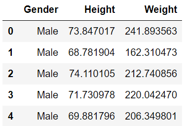

Next, check the number of observations and data types using .info( ) method. The dataset contains 10000 observations and the Gender variable is of object type while the other two (Weight and Height) are float type.

dataset.info()

1.2 Plotting histogram

Here, we will be going to use the height data for identifying the best distribution. So the first task is to plot the distribution using a histogram to get a preliminary idea of the distribution the data follows.

We will use the displot( ) function from the seaborn library to plot the histogram. The number of bins provided here is 100.

The plot shows that the height overall follows a normal distribution.

sns.set_style('white')
sns.set_context("paper", font_scale = 2)
sns.displot(data=dataset, x="Height", kind="hist", bins = 100, aspect = 1.5)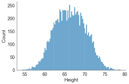

1.3 Data preparation

The next step is to prepare the data. Before we supply the data to Fitter we need to convert it to a NumPy array. One of the best ways to use the .values attribute on the height column (dataset[“Height”]) and saving it to the height variable.

height = dataset["Height"].values

1.4 Fitting distributions

The next step is to start fitting different distributions and finding out the best-suited distribution for the data.

The steps are:

1. Create a Fitter instance by calling the Fitter( )
2. Supply the data (height) and distributions list if you have a basic idea of the distributions that might fit your data
3. Apply the .fit( ) method
4. Generate the fitted distribution summary using .summary( ) method

Note:

If you have no initial idea about the distribution which might fit your data then you can call the Fitter( ) and supply the data (height) only.

The Fitter class in the backend uses the Scipy library which supports 80 distributions and the Fitter class will scan all of them, call the fit function for you, ignoring those that fail or run forever and finally give you a summary of the best distributions in the sense of sum of the square errors.

But this might take some time as it will try so many distributions and the fitting time also varies with your sample size. So, it is recommended to first plot a histogram and get an overall idea about the types of distributions that might fit the data and supply those distribution names in a list using the distributions argument. This will definitely save you time.

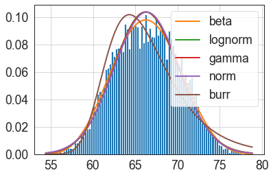
Here, I have fitted gamma, lognormal, beta, burr and normal distributions. Calling the summary( ) method on the fitted object shows the different distributions and fit statistics such as sumsquare_error, Akaike information criterion (aic) and Bayesian information criterion (bic) values. By default, the summary function ranks the best five distributions based on the sumsquare_error values in ascendingorder. Additionally, it provides an illustration of different distributions fitted over a histogram.

Based on the sumsquare_error value the best distribution for the height data is the beta distribution.

f = Fitter(height,
           distributions=['gamma',
                          'lognorm',
                          "beta",
                          "burr",
                          "norm"])
f.fit()
f.summary()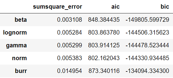

1.5 Identifying the best distribution

We can also retrieve the best distribution using the .get_best( ) method where we can also supply the method for selecting the best distribution. Here, we have supplied the sumsquare_error in the method argument as selection criteria. It will print the distribution name and corresponding parameters which has the lowest sumsquare_error.

We can see that the beta distribution is the best fit based on the sumsquare_error criteria. It also prints the optimized parameters for the beta distribution. It comprised of shape, scale and location parameters for beta distribution.

shape parameters (a, b) = [5.958, 6.498]
scale parameter (scale) = 52.872
location parameter (loc) = 28.213

f.get_best(method = 'sumsquare_error')

{‘beta’: (5.958303879012979,
6.498121982766356,
52.87268601986762,
28.21351507429388)}

1.6 Identifying the parameters

We can also print the fitted parameters using the fitted_param attribute and indexing it out using the distribution name [here, “beta”].

f.fitted_param["beta"]

(5.958303879012979, 6.498121982766356, 52.87268601986762, 28.21351507429388)

2. Fitting Distributions on a Randomly Drawn Data

Let’s see whether the Fitter( ) able to identify the distribution of random samples drawn from a distribution.

Let’s draw random samples from a normal (Gaussian) distribution using the NumPy module and then fit different distributions to see whether the fitter is able to identify the distribution.

2.1 Common distributions

Before we generate samples and fit distributions, one important thing to note is that the Fitter library also has a get_common_distribution( ) method which includes 10 common distributions. This could come in handy when you don’t have any idea about the distributions that might fit your data.

get_common_distributions()

[‘cauchy’, ‘chi2’, ‘expon’, ‘exponpow’, ‘gamma’, ‘lognorm’, ‘norm’, ‘powerlaw’, ‘rayleigh’, ‘uniform’]

2.2 Generating data from the normal distribution

Let’s draw 10000 random samples from a normal distribution using numpy’s random.normal( ) method. The method also require the mu (mean) and sigma (standard deviation). Here, we have provided mu = 0 and sigma = 0.1 in the sample generator.

mu, sigma = 0, 0.1 # mean and standard deviation
data = np.random.normal(mu, sigma, 10000)
data

array([ 0.05058757, 0.09303424, -0.14789721, …, -0.10781146,
-0.08059185, 0.09608844])

2.3 Fitting distributions

Next, fit the distributions using the Fitter( ) class and this time instead of supplying a list of distribution names we have supplied the common distributions using get_common_distributions( ). This will fit 10 common distributions as discussed in section 2.1.

The fitted distributions summary will provide top-five distributions that fit the data well. Based on the sumsquared_error criteria the best-fitted distribution is the normal distribution.

f = Fitter(data,
           distributions= get_common_distributions())
f.fit()
f.summary()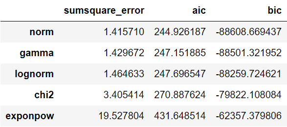

2.4 Get best-fitted distribution and parameters

Let’s check the parameters of the fitted normal distribution. The fitted normal distribution has correctly identified the mu and sigma values that we used for drawing random samples from the normal distribution.

f.get_best(method = 'sumsquare_error')

{‘norm’: (0.0005453480539770774, 0.10081629489894989)}

2.5 Get all supported distributions

You can print all supported distributions using the get_distribution( ) method.

Note: As the Fitter library uses Scipy for distribution fitting thus, it supports all distributions supported by the Scipy library.

get_distributions()

[‘alpha’, ‘anglit’, ‘arcsine’, ‘argus’, ‘beta’, ‘betaprime’, ‘bradford’, ‘burr’, ‘burr12’, ‘cauchy’, ‘chi’, ‘chi2’, ‘cosine’, ‘crystalball’, ‘dgamma’, ‘dweibull’, ‘erlang’, ‘expon’, ‘exponnorm’, ‘exponpow’, ‘exponweib’, ‘f’, ‘fatiguelife’, ‘fisk’, ‘foldcauchy’, ‘foldnorm’, ‘frechet_l’, ‘frechet_r’, ‘gamma’, ‘gausshyper’, ‘genexpon’, ‘genextreme’, ‘gengamma’, ‘genhalflogistic’, ‘geninvgauss’, ‘genlogistic’, ‘gennorm’, ‘genpareto’, ‘gilbrat’, ‘gompertz’, ‘gumbel_l’, ‘gumbel_r’, ‘halfcauchy’, ‘halfgennorm’, ‘halflogistic’, ‘halfnorm’,
‘hypsecant’, ‘invgamma’, ‘invgauss’, ‘invweibull’, ‘johnsonsb’, ‘johnsonsu’, ‘kappa3’, ‘kappa4’, ‘ksone’, ‘kstwo’, ‘kstwobign’, ‘laplace’, ‘levy’, ‘levy_l’, ‘levy_stable’, ‘loggamma’, ‘logistic’, ‘loglaplace’, ‘lognorm’, ‘loguniform’, ‘lomax’, ‘maxwell’, ‘mielke’, ‘moyal’, ‘nakagami’, ‘ncf’, ‘nct’, ‘ncx2’,
‘norm’, ‘norminvgauss’, ‘pareto’, ‘pearson3’, ‘powerlaw’, ‘powerlognorm’, ‘powernorm’, ‘rayleigh’, ‘rdist’, ‘recipinvgauss’, ‘reciprocal’, ‘rice’, ‘rv_continuous’, ‘rv_histogram’, ‘semicircular’, ‘skewnorm’, ‘t’, ‘trapz’, ‘triang’, ‘truncexpon’, ‘truncnorm’, ‘tukeylambda’, ‘uniform’, ‘vonmises’, ‘vonmises_line’, ‘wald’, ‘weibull_max’, ‘weibull_min’, ‘wrapcauchy’]

3. Streamlit Distribution Fitter Web Application

I have created a Streamlit based distribution fitter web app using the fitter library and deployed it on Heroku cloud — — -> link

You can play with it if you like…….Enjoy!

Note: If the app is in sleep mode it would take 30–45 seconds to reactivate, so have patience.

For more information on the Fitter library, you can read the documentation.

PDF documentation: link
Online documentation: link

Click here for the data and code

I hope you’ve found this article useful!

Rahul Raoniar

• If you enjoyed this, follow me on medium for more
• Connect with me on Twitter, LinkedIn, YouTube and Github

Featured image by Daniele Levis Pelusi on Unsplash