Rahul Raoniar
- posted on
- Comments Off on Survival Analysis in Python (KM Estimate, Cox-PH and AFT Model)
Introduction
Survival analysis is a branch of statistics for analysing the expected duration of time until one or more events occur. The method is also known as duration analysis or duration modelling, time-to-event analysis, reliability analysis and event history analysis.
The survival analysis is used to analyse following questions:
- A proportion of population surviving up to a given time
- Rate at which they are dying
- Understanding the impact of covariates on survival
The survival analysis is used in various field of research:
- Medical: Understanding patient’s survival when diagnosed with a deadly disease
- Medical: Hospital readmission duration after a major heart surgery
- Industry: When would Tesla car battery permanently die/fail
- Transportation: Waiting time of pedestrian after red (do-not walk) phase arrival at intersection
- E-commerce: After seeing ads when a person would purchase the product
- Human resource: When an employee would leave a company (churn)
There are various methods used by researchers to understand the time to event data. In this article, we are going to learn, the following types of models and try to understand their mechanism in time to event analysis.
- Kaplan-Maier Estimate (non-parametric)
- Cox Proportional Hazard Model (Semi-parametric)
- Accelerated Failure Time Model (Parametric)
Aim of the article
The aim of the article is to understand the survival of lung cancer patents using time to event analysis.
Note: If you are not familiar with the survival analysis, then I will highly recommend reading some articles and watching some YouTube videos on survival analysis. Here are few reading and video resources to learn about survival analysis:
Reading resources
Blog 1: Link
Blog 2: Link
Video Resources
1. Survival analysis concept videos (Channel: MarinStatsLectures-R Programming & Statistics): Link
2. Channel Zedstatistics: Link
**The current article presented an implementation of time to event analysis using Python’s Lifelines library.
Article Outline
- Description of lung cancer data
- Imputing missing values
- Kaplan Meier curve estimation
- Fitting Cox Proportional Hazard Regression
- Cox model results interpretation
- Testing Proportional Hazard assumption
- Fitting Accelerated Failure Time (AFT) Model
- AFT model results interpretation
Let’s start !!!!!!
Loading libraries
First, we need to install and load the following libraries to start with the survival analysis.
- Numpy: array manipulation
- Pandas: Data Manipulation
- Lifelines: Survival analysis
- Matplotlib: for plotting/generating graphs
import numpy as np
import pandas as pd
from lifelines import KaplanMeierFitter
import matplotlib.pyplot as plt
Lung Cancer Data
Next is to get an idea about the lung cancer data that we are going to use for the analysis. The data is originally available in R programming language (in survival library) [1]. So, I have downloaded it from R to use it for learning purpose. The data source is mentioned below.
Data Source: Loprinzi CL. Laurie JA. Wieand HS. Krook JE. Novotny PJ. Kugler JW. Bartel J. Law M. Bateman M. Klatt NE. et al. Prospective evaluation of prognostic variables from patient-completed questionnaires. North Central Cancer Treatment Group. Journal of Clinical Oncology. 12(3):601–7, 1994.
Data Description
The data consist of 228 observations and 10 variables/columns. The variable description is presented as the following:
- inst: Institution code
- time (d1): Survival time in days
- status (d2): censoring status 1 = censored, 2 = dead
- age (i1): Age in years
- sex (i2): Male = 1 Female = 2
- ph.ecog (i3): ECOG performance score as rated by the physician. 0 = asymptomatic, 1 = symptomatic but completely ambulatory, 2 = in bed <50% of the day, 3 = in bed > 50% of the day but not bed bound, 4 = bed bound
- ph.karno (i4): Karnofsky performance score (bad = 0; good = 100) rated by physician
- pat.karno (i4): Karnofsky performance score as rated by patient
- meal.cal (i5): Calories consumed at meals
- wt.loss (i6): Weight loss in last six months
Where: ‘i’ indicates the independent variables (covariates), and ‘d’ indicates dependent variables. Actually, the dependent variable or response is the time until the occurrence of an event (i.e., the lung cancer patient dies).
Data loading
First, let’s read the lung.csv data from our local storage and store in data object. We can print the first five observations using the head( ) function.
data = pd.read_csv("lung.csv", index_col = 0)
data.head()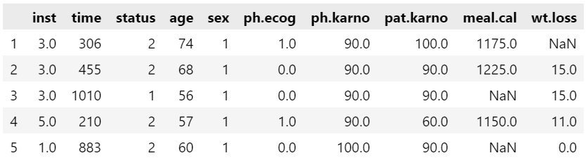
Next, let’s check the shape of the data using .shape attribute. The data consist of 228 observations and 10 variables/columns.
data.shape(228, 10)
Base label fixing
The status and sex are categorical data. The status consists of 1: censored and 2: dead; while, sex consist of 1: Male and 2 :Female. We can keep it like that, but I usually prefer the base label for categorical variable as 0 (zero). Thus, to make the base label 0 we need to deduct 1 from the variables.
data = data[['time', 'status', 'age', 'sex', 'ph.ecog', 'ph.karno','pat.karno', 'meal.cal', 'wt.loss']]
data["status"] = data["status"] - 1
data["sex"] = data["sex"] - 1
data.head()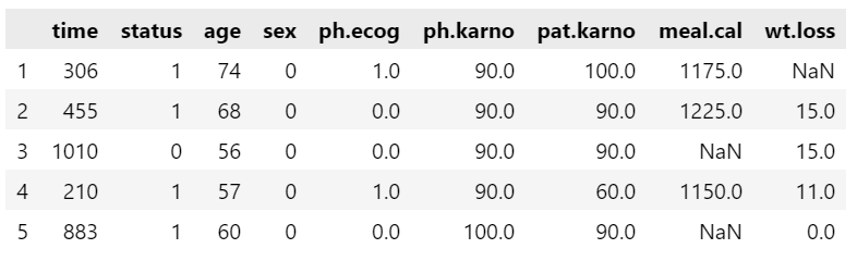
Now, let’s check the data type. Time, status, age, and sex are of integer64 type while ph.ecog, ph.karno, meal.cal and wt.loss are of float64 type.
data.dtypes
Checking and imputing missing values
The next important step is to check whether the variables contain missing values. We can check that using .isnull( ) method and by applying the .sum( ) over it. The resulting table illustrates the following:
ph.ecog: 1 missing value
ph.karno: 1 missing value
pat karno: 3 missing values
meal.cal: 47 missing values
wt.loss: 14 missing values
data.isnull().sum()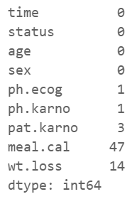
One-way to deal with missing values is to remove it entirely, but this will reduce the sample when you have already a small sample size. Next method would be to impute missing values with mean/median or with a particular value.
Instead of deleting missing observations here, I have imputed them (i.e., ph.karno, pat.karno, meal.cal and wt.loss) with the mean of the column as it is for demonstration purpose. Next, I removed the NA value of ph.ecog (a categorical column) using .dropna( ) method and converted it to int64.
data["ph.karno"].fillna(data["ph.karno"].mean(), inplace = True)
data["pat.karno"].fillna(data["pat.karno"].mean(), inplace = True)
data["meal.cal"].fillna(data["meal.cal"].mean(), inplace = True)
data["wt.loss"].fillna(data["wt.loss"].mean(), inplace = True)
data.dropna(inplace=True)
data["ph.ecog"] = data["ph.ecog"].astype("int64")
If you check the variables again, then you can see the variables now have no missing values. So, our data is now ready for initial analysis.
data.isnull().sum()
Now, the data contains 227 observations and 9 variables (as we did not select the institute variable).
data.shape(227, 9)
Data distribution
First, save the time variable in `T `and event/status variable in `E` that we will use during the model fitting process.
Let’s, plot a histogram of the time variable to get an overall idea of the distribution. The histogram shows that the time variable almost follows a Weibull or Log-normal distribution. We will check that during the AFT model estimation part.
T = data["time"]
E = data["status"]
plt.hist(T, bins = 50)
plt.show()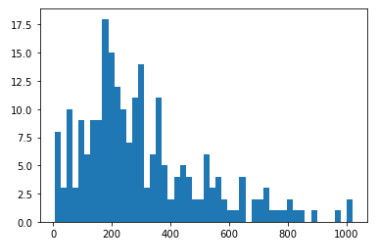
Kaplan-Maier Curve Estimation (Non-Parametric)
To start with survival analysis, the first step is to plot a survival curve of the overall data. It can be done by generating a Kaplan-Maier curve.
The Kaplan-Meier approach, also called the product-limit approach, is a popular approach which re-estimates the survival probability each time an event occurs. It is a non-parametric method, means it does not assume the distribution of the outcome variable (i.e., time).
Steps for generating KM curve:
step1: Instantiate KaplanMeierFitter( ) class object
step2: use .fit( ) method and supply duration = T and event_observed = E
step3: use plot_survival_function( ) to generate a KM curve
The curve illustrates how the survival probabilities changes over the time horizon. As the time passes, the survival probabilities of lung cancer patents reduces.
kmf = KaplanMeierFitter()
kmf.fit(durations = T, event_observed = E)
kmf.plot_survival_function()
We can generate the same plot without the 95% confidence interval using .survival_function_.plot() method.
kmf.survival_function_.plot()
plt.title('Survival function')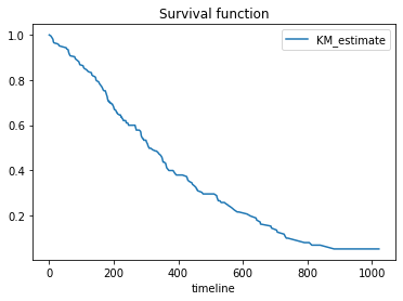
We can also plot a failure curve. It is just opposite of survival, i.e., Failure/death probabilities over time.
kmf.plot_cumulative_density()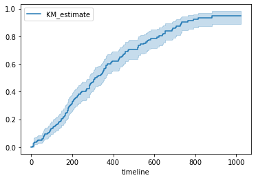
Median Survival Time and Confidence Intervals
The next step is to estimate the median survival time and 95% confidence intervals. This can be done using the .median_survival_time_ and median_survival_times( ). Here, the median survival time is 310 days, which indicates that 50% of the sample live 310 days and 50% dies within this time. The 95% CI lower limit is 284 days, while the upper limit is 361 days.
from lifelines.utils import median_survival_times
median_ = kmf.median_survival_time_
median_confidence_interval_ = median_survival_times(kmf.confidence_interval_)
print(median_)
print(median_confidence_interval_)
KM Plot for Gender/Sex Categories
Using the KM estimate, we can check the difference between categorical groups. Though, it is only viable when the variable has fewer categories. Here is an example where we are plotting the two survival curves, one for Male and another for Female.
The plot generation steps are:
- create an axis object
- create a mask (filtering object) “m” where males are true
- Fit and plot curves for Male and Female observations
The curve illustrates that the survival probabilities of female patients are overall higher compared to male patients at any instance of time.
ax = plt.subplot(111)
m = (data["sex"] == 0)
kmf.fit(durations = T[m], event_observed = E[m], label = "Male")
kmf.plot_survival_function(ax = ax)
kmf.fit(T[~m], event_observed = E[~m], label = "Female")
kmf.plot_survival_function(ax = ax, at_risk_counts = True)
plt.title("Survival of different gender group")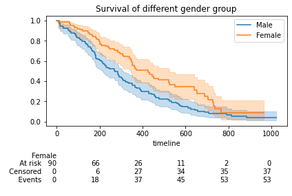
KM Plot for ph.ecog Categories
Similar to Gender/Sex, we can also plot separate survival curves for other categorical variables. Here, I have used a for loop that iterate over all ph.ecog categories and plot their survival function over a single plot.
The fourth plot (row 2, column 2) where the ecog == 3, looks incomplete.
ecog_types = data.sort_values(by = ['ph.ecog'])["ph.ecog"].unique()
for i, ecog_types in enumerate(ecog_types):
  ax = plt.subplot(2, 2, i + 1)
  ix = data['ph.ecog'] == ecog_types
  kmf.fit(T[ix], E[ix], label = ecog_types)
  kmf.plot_survival_function(ax = ax, legend = False)
  plt.title(ecog_types)
  plt.xlim(0, 1200)
plt.tight_layout()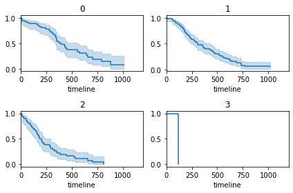
We can further investigate the ph.ecog == 3 using value_counts( ) method. It shows that the category 3 has only one observation which does not contribute much if we fit a model.
data['ph.ecog'].value_counts()
Thus, we need to remove this observation from the data. We can achieve this using a filtering process as shown below. Now, the dataset contains 226 observations and 9 variables.
data = data[data["ph.ecog"] != 3]
data.shape
(226, 9)
Let’s check the value count to reconfirm it. Now, it looks good, the 3rd category has been removed.
data['ph.ecog'].value_counts()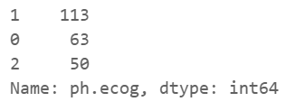
Cox Proportional Hazard Model (Semi-Parametric)
Cox-PH model is a semi-parametric model which solves the problem of incorporating covariates. In Cox’s proportional hazard model, the log-hazard is a linear function of the covariates and a population-level baseline hazard [2].

In the above equation, the first term is the baseline hazard and the second term known as partial hazard. The partial hazard inflates or deflates the baseline hazard based on covariates.
Cox-PH Model Assumptions
Cox proportional hazards regression model assumptions includes:
- Independence of survival times between distinct individuals in the sample
- A multiplicative relationship between the predictors and the hazard, and
- A constant hazard ratio over time
Definition of Hazard and Hazard Ratio
- Hazard is defined as the slope of the survival curve. It is a measure of how rapidly subjects are dying.
- The hazard ratio compares two groups. If the hazard ratio is 2.0, then the rate of deaths in one group is twice the rate in the other group.
Data Preparation
For fitting the Cox-PH model, we need to do some preprocessing of the categorical variables. Especially the dummy coding. The sex variable is binary, so we don’t have to dummy code it, until unless we want to alter the coding scheme, i.e., 0 for female and 1 for male. Here, we need to dummy code the ph.ecog variable only.
data.head()
Dummy Coding
We can dummy code the ph.ecog variable using pandas pd.get_dummies( ) method. I have added the prefix identifier for the generated columns. Here, we will consider the ecog_0 as the base category, so in next step we will remove it.
dummies_ecog = pd.get_dummies(data["ph.ecog"], prefix = 'ecog')
dummies_ecog.head(4)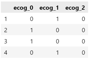
Concatenating with Original Data
Once dummy coding is done, we will concatenate the two columns, i.e., ecog_1 and ecog_2 column wise in our original dataset. Next, we need to drop the original categorical variable, i.e., ph.ecog using .drop( ) method.
dummies_ecog = dummies_ecog[["ecog_1", "ecog_2"]]
data = pd.concat([data, dummies_ecog], axis = 1)
data = data.drop("ph.ecog", axis = 1)
data.head()
Fitting Cox-PH Model
The next step is to fit the Cox-PH model.
The model fitting steps are:
- Instantiate CoxPHFitter( ) class object and save it in cph
- Call .fit( ) method and supply data, duration column and event column
- Print model estimate summary table
The summary table provides coefficients, exp(coef): also known as Hazard Ratio, confidence intervals, z and p-values.
from lifelines import CoxPHFitter
cph = CoxPHFitter()
cph.fit(data, duration_col = 'time', event_col = 'status')
cph.print_summary()
Interpretation of Cox-PH Model Results/Estimates
The interpretation of the model estimates will be like this:
- Wt.loss has a coefficient of about -0.01. We can recall that in the Cox proportional hazard model, a higher hazard means more at risk of the event occurring. Here, the value of exp(-0.01) is called the hazard ratio.
- It shows that a one unit increase in wt loss means the baseline hazard will increase by a factor of exp(-0.01) = 0.99 ⇾ about a 1% decrease.
- Similarly, the values in the ph.ecog column are: [0 = asymptomatic, 1 = symptomatic but completely ambulatory and 2 = in bed <50% of the day]. The value of the coefficient associated with ecog2, exp(1.20), is the value of ratio of hazards (Hazard Ratio) associated with being “in bed <50% of the day (coded as 2)” compared to asymptomatic (coded as 0, base category). This indicates the risk (rate) of dying is 3.31 times for patients who are “in bed <50% of the day” compared to asymptomatic patients.
Plot Coefficients
Next we can plot the ranking of variables in terms of their log(HR) using the .plot( ) method.
plt.subplots(figsize = (10, 6))
cph.plot()
Plot Partial Effects on Outcome (Cox-PH Regression)
We can use our fitted model to see how the survival changes as we change the covariate values. Here, I have used the plot_partial_effects_on_outcome( ) method to see how the survival varies for age group of 50, 60, 70 and 80 years old patents compared to their baseline function. It clearly highlights that young patents has higher survival probabilities at any given instance of time compared to old patients.
cph.plot_partial_effects_on_outcome(covariates = 'age', values = [50, 60, 70, 80], cmap = 'coolwarm')
Check Proportional Hazard Assumption
Once we fit the model, the next step is to verify the proportional hazard assumption. We can directly use the check_assumptions( ) method that return a log rank test statistics.
The null (H0) hypothesis assumed that the proportional hazard criteria satisfied, while alternative hypothesis (H1) infer that the proportional hazard assumption criteria not met (violated).
cph.check_assumptions(data, p_value_threshold = 0.05)
We can also use the proportional_hazard_test( ) method to perform the same.
The result revealed that at 5% significance level, only meal.cal violated the assumption. There are various approach to deal with it, for example we can convert it to a binned category, or we can use a parametric Cox-PH model.
from lifelines.statistics import proportional_hazard_test
results = proportional_hazard_test(cph, data, time_transform='rank')
results.print_summary(decimals=3, model="untransformed variables")
Accelerated Failure Time (AFT) Model
If the proportional hazard assumption criteria of Cox-PH model is not satisfied, in such instance, a better approach is to use a parametric model. Accelerated Failure Time (AFT) is one of the popular parametric model used in survival analysis.
The model assumes that the survival function follows a parametric continuous distribution. For instance, one can assume a Weibull distribution or a Log-normal distribution.
The parametric AFT model assumes that survival function that derived from say two population (for example P and Q) are related by some acceleration factor lambda (λ), which can be modelled as a function of covariates.
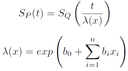
Based on the covariates, the AFT model can accelerate or decelerate the failure times. The AFT model coefficients can be interpreted easily: a unit increase in a covariate means the average/median survival time changes by a factor of exp(b_i) [2].
Identifying the Best Fitted Distribution
There are many distributions exist that we can fit. So, the first step is to identify the best distribution that best fits the data. The common distributions are Weibull, Exponential, Log-Normal, Log-Logistic and Generalized Gamma.
Here is a step-by-step guide for identifying best fitted distribution:
- Import distributions from lifelines library
- Instantiate the class object and save inside a variable. For example, here the Weibull class object has been saved inside “wb”
- Iterate through all model objects and fit with the time and event data
- Print the AIC value
- The distribution with the lowest AIC value presents the best fitted distribution
Here, the Weibull provided the lowest AIC (2286.4) value thus, it can be selected as best fitted distribution for our AFT model.
from lifelines import WeibullFitter,\
                      ExponentialFitter,\
                      LogNormalFitter,\
                      LogLogisticFitter
# Instantiate each fitter
wb = WeibullFitter()
ex = ExponentialFitter()
log = LogNormalFitter()
loglogis = LogLogisticFitter()
# Fit to data
for model in [wb, ex, log, loglogis]:
    model.fit(durations = data["time"], event_observed = data["status"])
# Print AIC
print("The AIC value for", model.__class__.__name__, "is",  model.AIC_)
Fitting Weibull AFT Model
The next step is to fit the Weibull Fitter class with the lung cancer data and print the summary. The model estimate provides coefficients, exp(coef) also known as Acceleration Factor/ Time Ratio, confidence intervals, z statistics and p-values.
from lifelines import WeibullAFTFitter
weibull_aft = WeibullAFTFitter()
weibull_aft.fit(data, duration_col='time', event_col='status')
weibull_aft.print_summary(3)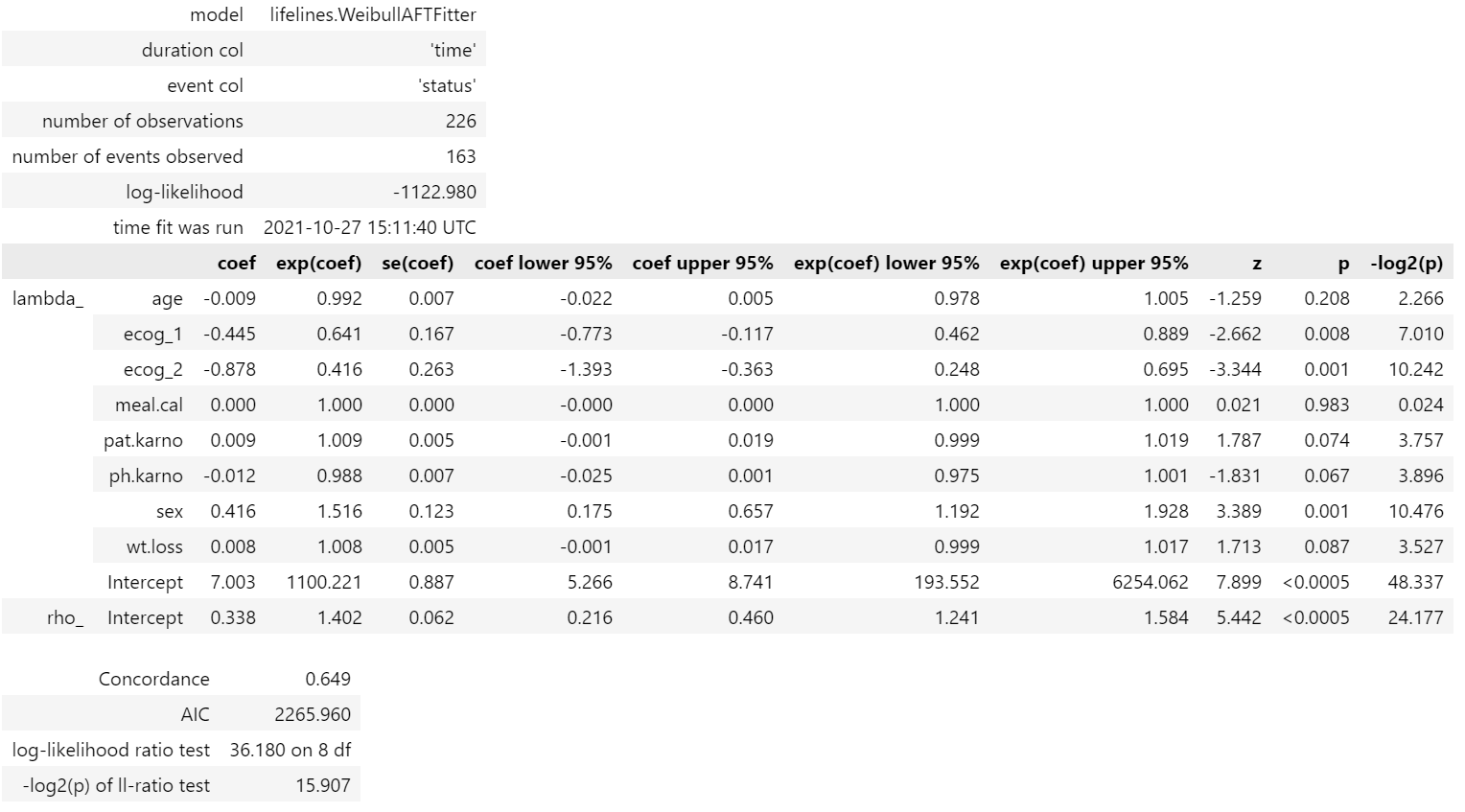
Interpretation of AFT Model Results/Estimates
The step-by-step interpretation of the AFT model is described below:
- A unit increase in covariate indicates that the mean/median survival time will change by a factor of exp(coefficient).
- If the coefficient is positive, then the exp(coefficient) will be >1, which will decelerate the incident/event time. Similarly, a negative coefficient will reduce the mean/median survival time.
Example:
- Sex, which contains [0: Male (base) and 1: Female], has a positive coefficient.
- This means being a female subject compared to male changes mean/median survival time by exp(0.416) = 1.516, approximately a 52% increase in mean/median survival time.
Median and Mean Survival Time
We can estimate the mean and median survival time using mean_survival_time_ and median_survival_time_ attributes.
print(weibull_aft.median_survival_time_)
print(weibull_aft.mean_survival_time_)
419.097
495.969
Plotting Coefficients
Next, we can plot the ranking of variables in terms of their log(accelerated failure rate) using the .plot( ) method.
plt.subplots(figsize=(10, 6))
weibull_aft.plot()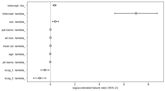
Plot Partial Effects on Outcome (Weibull Regression)
We can use our fitted model to see how the survival changes as we change the covariate values. Here, I have used the plot_partial_effects_on_outcome( ) method to see how the survival varies among 50, 60, 70 and 80 years old patents compared to their baseline function. It clearly highlights that young patents has higher survival probabilities at any given instance of time compared to old patients.
plt.subplots(figsize=(10, 6))
weibull_aft.plot_partial_effects_on_outcome('age', range(50, 80, 10), cmap='coolwarm')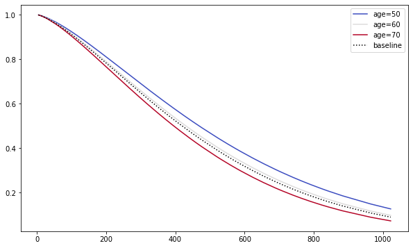
Survival analysis is a powerful technique for conducting time to event analysis. I hope this article give you enough motivation to try it with your collected data.
Click here for the data and code
References
[1] Loprinzi CL. Laurie JA. Wieand HS. Krook JE. Novotny PJ. Kugler JW. Bartel J. Law M. Bateman M. Klatt NE. et al. Prospective evaluation of prognostic variables from patient-completed questionnaires. North Central Cancer Treatment Group. Journal of Clinical Oncology. 12(3):601–7, 1994.
[2] Davidson-Pilon, (2019). lifelines: survival analysis in Python. Journal of Open Source Software, 4(40), 1317, https://doi.org/10.21105/joss.01317
I hope you’ve found this article useful!