In the supervised machine learning world, there are two types of algorithmic tasks often performed. One is called regression (predicting continuous values) and the other is called classification (predicting discrete values). In this blog, I have presented an example of a binary classification algorithm called “Binary Logistic Regression” which comes under the Binomial family with a logit link function. Binary logistic regression is used for predicting binary classes. For example, in cases where you want to predict yes/no, win/loss, negative/positive, True/False and so on.

This blog will guide you through a process of how to use tidymodels package to fit and evaluate model performance with very few easy steps.

Article Outline

• Data Background
• Aim of the modelling
• Libraries and Data Loading
• Setting reference level
• Generating train and test split
• Model Fitting/Training
• Interpretation of Model Summary
• Model Evaluation on Test data Set
• References

Data Background

In this example, we are going to use the Pima Indian Diabetes 2 data set obtained from the UCI Repository of machine learning databases (Newman et al. 1998).

This data set is originally from the National Institute of Diabetes and Digestive and Kidney Diseases. The objective of the data set is to diagnostically predict whether or not a patient has diabetes, based on certain diagnostic measurements included in the data set. Several constraints were placed on the selection of these instances from a larger database. In particular, all patients here are females at least 21 years old of Pima Indian heritage.

The Pima Indian Diabetes 2 data set is the refined version (all missing values were assigned as NA) of the Pima Indian diabetes data. The data set contains the following independent and dependent variables.

Independent variables (symbol: I)

• I1: pregnant: Number of times pregnant
• I2: glucose: Plasma glucose concentration (glucose tolerance test)
• I3: pressure: Diastolic blood pressure (mm Hg)
• I4: triceps: Triceps skinfold thickness (mm)
• I5: insulin: 2-Hour serum insulin (mu U/ml)
• I6: mass: Body mass index (weight in kg/(height in m)\²)
• I7: pedigree: Diabetes pedigree function
• I8: age: Age (years)

Dependent Variable (symbol: D)

• D1: diabetes: diabetes case (pos/neg)

Aim of the Modelling

• fitting a binary logistic regression machine learning model using tidymodels library
• testing the trained model’s prediction (model evaluation) strength on the unseen/test data set using various evaluation metrics.

Loading Libraries and Datasets

Step1: At first we need to install the following packages using install.packages( ) function and loading them using library( ) function.

library(mlbench)     # for PimaIndiansDiabetes2 dataset
library(tidymodels)  # for model preparation and fitting

Step2: Next, we need to load the data set from the mlbench package using the data( ) function.

After data loading, the next essential step is to perform an exploratory data analysis, which will help in data familiarization. Use the head( ) function to view the top six rows of the data.

data(PimaIndiansDiabetes2)
head(PimaIndiansDiabetes2)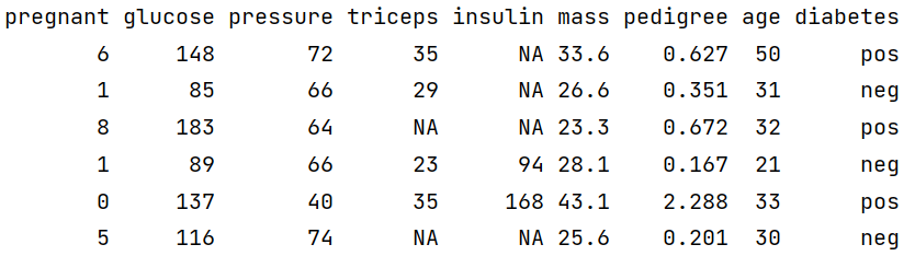

The Diabetes data set has 768 observations and 9 variables. The first 8 variables are numeric/double type and the dependent/output variable is of factor/categorical type. It is also noticeable many variables contain NA values. So our next task is to refine/modify the data so that it gets compatible with the modelling algorithm.

# See the data strcuture 
glimpse(PimaIndiansDiabetes2)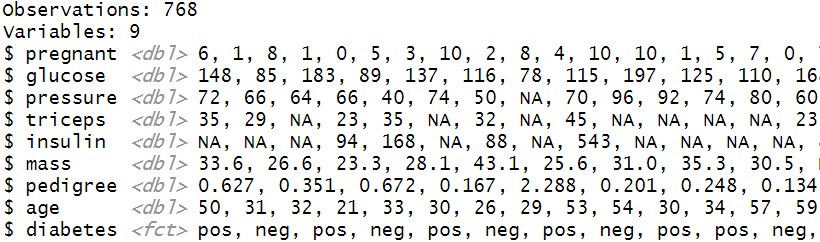

Data Preparation

The first step is to remove data rows with NA values using na.omit( ) function. The next step is to check the refined version of the data using glimpse( ) function.

Diabetes <- na.omit(PimaIndiansDiabetes2) #removing NA values
glimpse(Diabetes)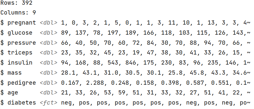

The final (prepared) data contains 392 observations and 9 columns. The independent variables are numeric/double type, while the dependent/output binary variable is of factor/category type (neg/ pos).

Data levels

We can check the reference level of the dependent variable using the levels( ) function. We can observe that the reference level is neg (the very first level).

levels(Diabetes$diabetes)

Setting Reference Level

For better interpretation (later for ROC curve plotting) we need to fix the reference level of our dependent variable “diabetes” to positive (pos) using the relevel( ) function.

Diabetes$diabetes <- relevel(Diabetes$diabetes, ref = "pos")
levels(Diabetes$diabetes)

Train and Test Split

The whole data set generally split into 75% train and 25% test data set (general rule of thumb). 75% of the training data is being used for model training, while the rest 25% is used for checking how the model generalized on unseen/test data set.

To create a split object you can use the initial_split( ) function where you need to supply the dataset, proportion and a strata argument. Supplying your dependent variable in the strata attribute performs stratified sampling. Stratifed sampling is helpful if your dependent variable has a class imbalance.

The next step is to call the training( ) and testing( ) functions on the split object (i.e., diabetes_split) to save the train (diabetes_train) and test (diabetes_test) datasets.

The training samples include 295 observations while testing samples include 97 observations.

set.seed(123)
# Create data split for train and test
diabetes_split <- initial_split(Diabetes,
                                prop = 0.75,
                                strata = diabetes)

# Create training data
diabetes_train <- diabetes_split %>%
                    training()

# Create testing data
diabetes_test <- diabetes_split %>%
                    testing()
# Number of rows in train and test dataset
nrow(diabetes_train)
nrow(diabetes_test)

[1] 295

[1] 97

Fitting Logistic Regression

You can fit any type of model (supported by tidymodels) using the following steps.

Step 1: call the model function: here we called logistic_reg( ) as we want to fit a logistic regression model.

Step 2: use set_engine( ) function to supply the family of the model. We supplied the “glm” argument as Logistic regression comes under the Generalized Linear Regression family.

Step 3: use set_mode( ) function and supply the type of model you want to fit. Here we want to classify pos vs neg, so it is a classification.

Step 4: Next, you need to use the fit( ) function to fit the model and inside that, you have to provide the formula notation and dataset (diabetes_train).

plus notation →
diabetes ~ ind_variable 1 + ind_variable 2 + …….so on

tilde dot notation →

diabetes~.

means diabetes is predicted by the rest of the variables in the data frame (means all independent variables) except the dependent variable i.e., diabetes.

After model fitting, the next step is to generate the model summary table. You can produce a beautiful summary table using the tidy( ) function of the broom library (which comes inbuilt with tidymodels library). The reported coefficients are in log-odds terms.

fitted_logistic_model<- logistic_reg() %>%
        # Set the engine
        set_engine("glm") %>%
        # Set the mode
        set_mode("classification") %>%
        # Fit the model
        fit(diabetes~., data = diabetes_train)
tidy(fitted_logistic_model)    # Generate Summary Table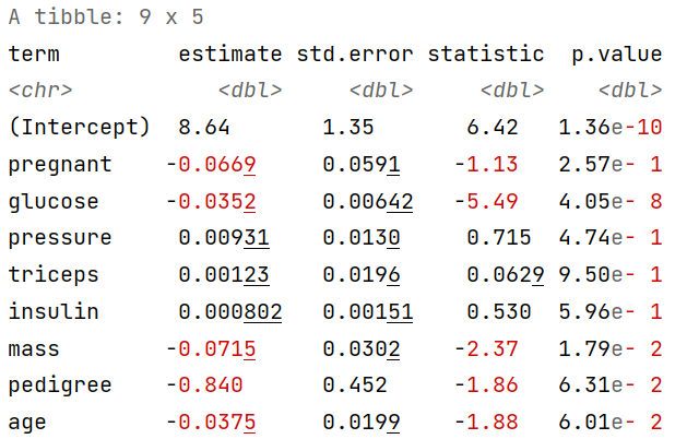

Note: The coefficients’ sign and value would change based on the reference you set for the dependent variable (in our case pos is the reference level) and the observation you have got in the training sample based on the random sampling selection process [the above results are just an example].

Odds Ratio

The interpretation of coefficients in the log-odds term does not make much sense if you need to report it in your article or publication. That is why the concept of odds ratio was introduced.

The ODDS is the ratio of the probability of an event occurring to the event not occurring. When we take a ratio of two such odds it called Odds Ratio.

Mathematically, one can compute the odds ratio by taking the exponent of the estimated coefficients. For example, you can get directly the odds ratios of the coefficient by supplying the exponentiate = True inside the tidy( ) function.

The produced result solely dependent on the samples that we have got during the splitting process. You might get a different result (odds ratio values).

tidy(fitted_logistic_model, exponentiate = TRUE)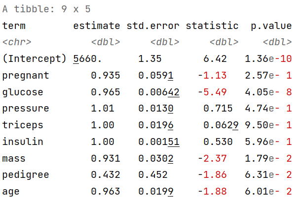

Significant Odds

The table produced by tidy( ) function can be filtered. Here we filtered out the variables whose p-values are less than 0.05 (5%) significant level. For our sample glucose and mass has a significant impact on diabetes.

tidy(fitted_logistic_model, exponentiate = TRUE) %>%
  filter(p.value < 0.05)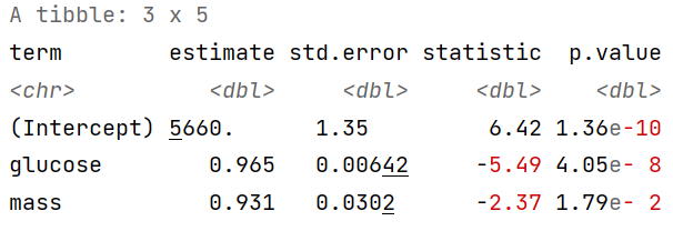

Model Prediction

Test Data Class Prediction

The very next step is to generate the test predictions that we could use for model evaluation. To generate the class prediction (pos/ neg) we can use the predict function and supply the trained model object, test dataset and the type which is here “class” as we want the class prediction, not probabilities.

# Class prediction
pred_class <- predict(fitted_logistic_model,
                      new_data = diabetes_test,
                      type = "class")

pred_class[1:5,]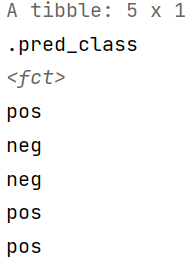

Test Data Class Probabilities

We can also generate predictions for the class probabilities by supplying the “prob” argument in the type attribute.

# Prediction Probabilities
pred_proba <- predict(fitted_logistic_model,
                      new_data = diabetes_test,
                      type = "prob")

pred_proba[1:5,]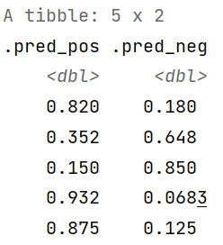

Final Data Preparation for Model Evaluation

The next step is to prepare a data frame that includes the diabetes column from the original test dataset, predicted class and class prediction probabilities. We will be going to use this data frame for model evaluation.

diabetes_results <- diabetes_test %>%
  select(diabetes) %>%
  bind_cols(pred_class, pred_proba)

diabetes_results[1:5, ]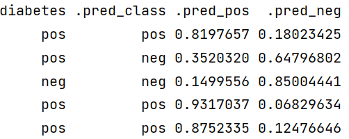

Model Evaluation

Confusion Matrix

We can generate a confusion matrix by using the conf_mat( ) function by supplying the final data frame i.e., diabetes_results, the truth column i.e., diabetes and predicted class (.pred_class) in the estimate attribute.

The confusion matrix revealed that the test dataset has 65 sample cases of negative (neg) and 32 cases of positive (pos) observations. The trained model classified 61 negatives (neg) and 18 positives (pos) class, accurately.

conf_mat(diabetes_results, truth = diabetes,
         estimate = .pred_class)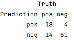

We can also use the yardstick package which comes with tidymodels package to generate different evaluation metrics for the test data set.

Accuracy

We can calculate the classification accuracy by using the accuracy( ) function by supplying the final data frame i.e., diabetes_results, the truth column i.e., diabetes and predicted class (.pred_class) in the estimate attribute. The model classification accuracy on test dataset is about 81.4%.

accuracy(diabetes_results, truth = diabetes,
         estimate = .pred_class)

Sensitivity

The sensitivity of a classifier is the ratio between how much were correctly identified as positive to how much were actually positive.

Sensitivity = TP / FN+TP

The estimated sensitivity value is 0.562 indicating poor detection of positive classes in the test dataset.

sens(diabetes_results, truth = diabetes,
    estimate = .pred_class)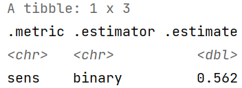

Specificity

Specificity of a classifier is the ratio between how much were correctly classified as negative to how much was actually negative.

Specificity = TN/FP+TN.

The estimated specificity value is 0.938 indicating overall good detection of negative classes in the test dataset.

spec(diabetes_results, truth = diabetes,
    estimate = .pred_class)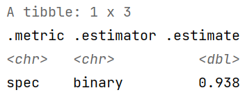

Precision

How much were correctly classified as positive out of all positives?

Precision = TP/TP+FP

The estimated precision value is 0.818.

precision(diabetes_results, truth = diabetes,
    estimate = .pred_class)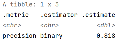

Recall

Recall and sensitivity are one and the same.

Recall = TP / FN+TP

The estimated recall value is 0.562.

recall(diabetes_results, truth = diabetes,
      estimate = .pred_class)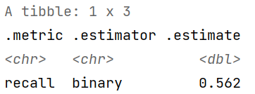

F-measure

F-measure is a weighted harmonic mean of precision and recall with the best score of 1 and the worst score of 0. F-measure score conveys the balance between precision and recall. The F1 score is about 0.667, which indicates that the trained model has a classification strength of 66.7%.

f_meas(diabetes_results, truth = diabetes,
       estimate = .pred_class)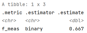

Kappa

Cohen Kappa gives information on how much better a model over the random classifier. Kappa can range from −1 to +1. The value <0 means no agreement while 1.0 shows perfect agreement. The estimated kappa statistics revealed a moderate agreement.

kap(diabetes_results, truth = diabetes,
    estimate = .pred_class)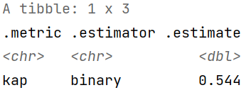

Matthews Correlation Coefficient (MCC)

The Matthews correlation coefficient (MCC) is used as a measure of the quality of a binary classifier. The value ranges from −1 and +1.

MCC: -1 indicates total disagreement
MCC: 0 indicate no agreement
MCC: +1 indicates total aggrement

The estimated MCC statistics revealed a moderate agreement.

mcc(diabetes_results, truth = diabetes,
    estimate = .pred_class)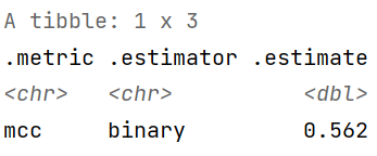

Custom Metrics

We can use custom_metrics( ) function to generate multiple evaluation metrics.

Step 1: generate a custom metric set using metric_set( )Step 2: use the custom_metrics( ) function and supply the diabetes_results data frame, diabaets column and predicted class (.pred_class).

custom_metrics <- metric_set(accuracy, sens, spec, precision, recall, f_meas, kap, mcc)
custom_metrics(diabetes_results,
               truth = diabetes,
               estimate = .pred_class)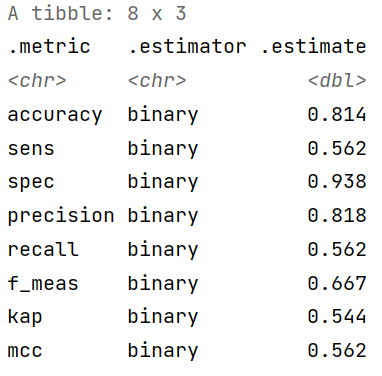

ROC-AUC

ROC-AUC is a performance measurement for the classification problem at various thresholds settings. ROC_AUC tells how much the model is capable of distinguishing between classes. The trained logistic regression model has a ROC-AUC of 0.921 indicating overall good predictive performance.

roc_auc(diabetes_results,
        truth = diabetes,
        .pred_pos)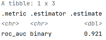

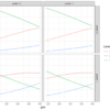
ROC Curve

The ROC curve is plotted with TPR/Recall/Sensitivity against the FPR/ (1- Specificity), where TPR is on the y-axis and FPR is on the x-axis. A line is drawn diagonally to denote 50–50 partitioning of the graph. If the curve is more close to the line, lower the performance of the classifier, which is no better than a mere random guess.

You can generate a ROC Curve using the roc_curve( ) function where you need to supply the truth column (diabetes) and predicted probabilities for the positive class (.pred_pos).

Our model has got a ROC-AUC score of 0.921 indicating a good model that can distinguish between patients with diabetes and no diabetes.

diabetes_results %>%
  roc_curve(truth = diabetes, .pred_pos) %>%
  autoplot()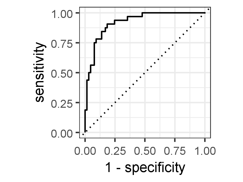

Binary logistic regression is still a vastly popular ML algorithm (for binary classification) in the STEM research domain. It is still very easy to train and interpret, compared to many sophisticated and complex black-box models.

Note:

In the second blog, we will learn how to perform feature engineering such as removing correlated features, dummy coding of categorical features and, applying transformations using the tidymodels library.

Dataset and Code

Click here for diabetes data and code