One Zero Blog

Introduction

The Apache Spark is a fast and powerful framework that provides an API to perform massive distributed processing over resilient sets of data. It also ensures data processing with lightning speed and supports various languages like Scala, Python, Java, and R.

PySpark is the Python API for using Apache Spark, which is a parallel and distributed engine used to perform big data analytics. In the era of big data, PySpark is extensively used by Python users for performing data analytics on massive datasets and building applications using distributed clusters.

In this article, we will get familiar with the basic functionality of PySpark, especially with the data manipulation part. Here, we will learn how to load data, explore it, handle missing values, perform filtering operations and applying aggregations over different groups of data.

Article Outline

1. Loading Dataset Into PySpark
2. Exploring Data Frame
3. Handling Missing Values
4. Filtering Operations
5. Group by and Aggregate

Dataset Description

In this blog, we’re primarily going to use Tips dataset [a small dataset] just for demonstration purpose. The data was reported in a collection of case studies for business statistics. The dataset is also available through the Python package Seaborn.

Source:
Bryant, P. G. and Smith, M. A. (1995), Practical Data Analysis: Case Studies in Business Statistics, Richard D. Irwin Publishing, Homewood, IL.

The Tips data contains 244 observations and 7 variables (excluding the index). The variables descriptions are as follows:

bill: Total bill (cost of the meal), including tax, in US dollars
tip: Tip (gratuity) in US dollars
sex: Sex of person paying for the meal (Male, Female)
smoker: Presence of smoker in a party? (No, Yes)
weekday: day of the week (Saturday, Sunday, Thursday and Friday)
time: time of day (Dinner/Lunch)
size: the size of the party

1. Loading Dataset Into PySpark

Loading libraries

The first step would be to install and load Pyspark and Pandas libraries that we will need to perform data loading and manipulations.

# pip install pyspark 
# or
# conda install pyspark if using anaconda distribution
import pyspark
from pyspark.sql import SparkSession
import pandas as pd

Creating a Spark Session

The next step is to create a PySpark session using SparkSession.builder.appName and instantiating with getOrCreate( ).

If you print the session object, it will show that we are using PySpark version 3.1.2.

spark = SparkSession.builder.appName("Introduction to Spark").getOrCreate()
spark

Loading dataset to PySpark

To load a dataset into Spark session, we can use the spark.read.csv( ) method and save inside df_pyspark. If we print the df_pyspark object, then it will print the data column names and data types. We can observe that PySpark read all columns as string, which in reality not the case. We will fix it soon.

df_pyspark = spark.read.csv("tips.csv")
df_pyspark

To print a data frame using PySaprk we need to use the show( ) method and pass the number of rows we want to print as an integer value.

df_pyspark.show(5)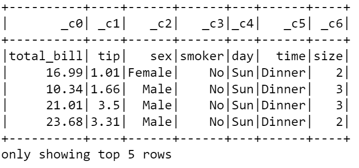

Print Data Types

Like pandas dtypes, PySpark has an inbuilt method printSchema( ), which can be used to print the data types.

df_pyspark.printSchema()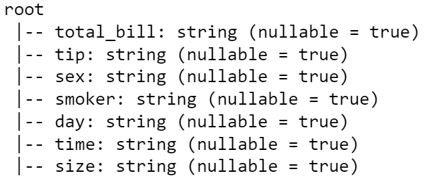

Correct Way to Read Dataset

The better way to read a csv file is using the spark.read.csv( ) method, where we need to supply the header = True if the column contains any name. Further, we need to supply the inferSchema = True argument so that while reading data, it infers the actual data type.

df_pyspark = spark.read.csv("tips.csv", header = True, inferSchema = True)
df_pyspark.show(5)

Print Data Types

If we now print the Schema it will show that the total_bill and tip variables are of double data type, the size variable is of integer type and the rest are string type.

df_pyspark.printSchema()

Let’s see the data type of the data object that we saved inside df_pyspark. It is a sql.dataframe.DataFrame. So, we can apply various functionality on this data set offered by Pandas library.

type(df_pyspark)

pyspark.sql.dataframe.DataFrame

We can print column names using the .column attribute. The dataset contains seven columns, i.e., ‘total_bill’, ‘tip’, ‘sex’, ‘smoker’, ‘day’, ‘time’ and ‘size’.

df_pyspark.columns

[‘total_bill’, ‘tip’, ‘sex’, ‘smoker’, ‘day’, ‘time’, ‘size’]

You can use pandas head( ) method, but it will print the rows as a list.

df_pyspark.head(3)

2. Exploring DataFrame

Let’s proceed with the data frames. The data frame object in PySpark act similar to pandas dataframe, but PySpark adds many additional functionalities that makes data manipulation easy and fun. Let’s visit a few everyday functionalities that we usually perform with pandas.

Selecting columns

The first thing we often do is selecting and printing columns. Let’s say we want to select the “sex” column. We can do this using select( ) method. To view it, we need to add the show( ) method.

df_pyspark.select("sex").show(5)

What if we want to view multiple columns at once. We can do that by passing the column names as a list inside the select( ) function.

Note: this select functionality reminds us of the dplyr package of R programming language and SQL.

df_pyspark.select(["tip", "sex"]).show(5)

We can achieve the column selection also by providing select(df[column index]) notation inside the select( ) method.

df_pyspark.select(df_pyspark[1], df_pyspark[2]).show(5)

Describe Data Frame

Similar to pandas, PySpark also supports describe( ) method which provides count, mean, standard deviation, min, and max.

df_pyspark.describe().show()

Generating a New Column

To generate a new column, we need to use the withcolumn( ) method, which takes the new column name as first argument and then the computation [here we computed the ratio of tip and total_bill).

df_pyspark = df_pyspark.withColumn("tip_bill_ratio", (df_pyspark["tip"]/df_pyspark["total_bill"])*100)
df_pyspark.show(5)

Dropping Columns

To drop a column, we need to use the .drop( ) method and pass the single column name or column names as a list [in case we want to drop multiple columns]. Here, we have dropped the “tip_bill_ratio” column.

df_pyspark = df_pyspark.drop("tip_bill_ratio")
df_pyspark.show(5)

Rename Columns

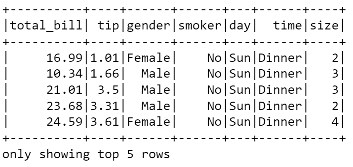
To rename a column, we need to use the withColumnRenamed( ) method and pass the old column as first argument and new column name as second argument.

df_pyspark.withColumnRenamed("sex", "gender").show(5)

If you want to rename multiple columns at once, then you need to chain the withColumnRenamed( ) method one after another.

df_pyspark.withColumnRenamed("sex", "gender").withColumnRenamed("time", "event").show(5)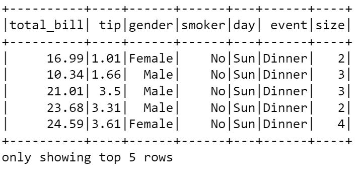

3. Handling Missing Values

Let’s learn how to handle missing values in PySpark. Similar to Pandas, PySpark also comes with build in methods to handle missing values.

Load the Data Frame with Missing Values

Before we begin handling missing values, we require loading a separate tips dataset with missing values. The missing values are denoted using null.

df_pyspark = spark.read.csv("tips_missing.csv", header = True, inferSchema = True)
df_pyspark.show(20)

Removing observations with null values

Let’s start with the easiest one, where say we want to drop any observation (row) where any of the cell contains a missing value. We could do that by using the .na.drop( ) method. Remember that to view it we need to add the .show( ) method.

df_pyspark.na.drop().show()

The drop( ) method contains a how argument. In the above example, by default, how was set to “any” (how = “any”), which means it will drop any observation that contains a null value.

### how == any
df_pyspark.na.drop(how = "any").show()

If we set how = “all”, it will delete an observation if all the values are null. For example, in out tips_missing.csv dataset, the 3rd observation contained all null values. We can see that after applying how = “all” using drop( ), now it has dropped from the data frame.

### how == all
df_pyspark.na.drop(how = "all").show()

Setting Threshold

The .drop( ) method also contains a threshold argument. This argument indicates that how many non-null values should be there in an observation (i.e., in a row) to keep it.

df_pyspark.na.drop(how = "any", thresh = 2).show()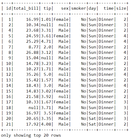

Subset

The subset argument inside the .drop( ) method helps in dropping entire observations [i.e., rows] based on null values in columns. For a particular column where null value is present, it will delete the entire observation/row.

df_pyspark.na.drop(how = "any", subset = ["tip"]).show()

The next part is related to dealing with missing values.

Filling null Values

Dealing with missing values is easy in PySpark. Let’s say we want to fill the null values with string “Missing”. We can do that by using .na.fill(“Missing”) notation. This going to fill only the null values of columns with string type.

### Replaces string column values
df_pyspark.na.fill("Missing").show()

Similarly, if we supply a numeric value, then it will replace the values in the numeric columns.

### Replaces numeric column values
df_pyspark.na.fill(3).show()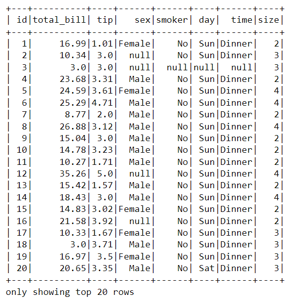

We can also specify the column names explicitly to fill missing values by supplying the column names inside a square brackets. Like here, we supplied [“sex”, “day”] inside the fill( ) method.

df_pyspark.na.fill("Missing", ["sex", "day"]).show()

Imputing Missing Values with Column Mean/Average

We often need to impute missing values with column statistics like mean, median and standard deviation. To achieve that the best approach will be to use an imputer.

Step1: import the Imputer class from pyspark.ml.feature

Step2: Create an Imputer object by specifying the input columns, output columns, and setting a strategy (here: mean).

Note: The outputCols contains a list comprehension.

Step3: fit and transform the data frame using the imputer object.

This will create two different columns with imputed mean values.

### Filling with mean values with an imputer
from pyspark.ml.feature import Imputer
### Create an imputer object
imputer = Imputer(
          inputCols= ["total_bill", "tip"],
          outputCols = ["{}_imputed".format(c) for c in ["total_bill", "tip"]]
    ).setStrategy("mean")
### Fit imputer on Data Frame and Transform it
imputer.fit(df_pyspark).transform(df_pyspark).show()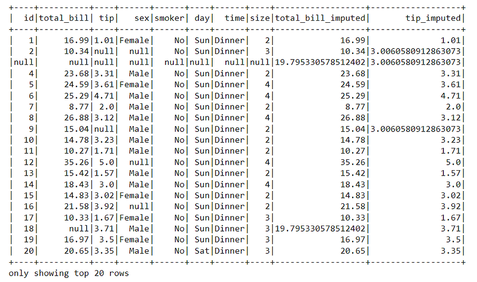

4. Filtering Operations

We often use filtering to filter out a chunk of data that we need for a specific task. PySpark’s .filter( ) method makes is very easy to filter data frames.

Let’s say we want to filter the observations where tip ≤ 2.To achieve this, we need to supply the condition inside .filter( ) method using a quotation.

# Find tips less than or equal to 2
df_pyspark.filter("tip <= 2").show(5)

After performing the filter operation, we can subsequently perform a selection operation to separate out specific columns.

df_pyspark.filter("tip <= 2").select(["total_bill", "tip"]).show(5)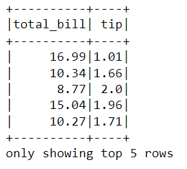

We can perform multiple conditional filtering, separating by an OR (|) or AND (&) operators. While using multiple filtering, it is recommended to enclose them using parenthesis ( ).

### Two filtering conditions
df_pyspark.filter((df_pyspark["tip"] <= 1) | (df_pyspark["tip"] >= 5)).select(["total_bill", "tip"]).show(5)

We can call for just the opposite what the actual filtering condition indented for using a tilde ~ sign in front of the filtering code. Here in the below code, it means that ignore observations where tip ≤ 2.

### Not operation
df_pyspark.filter(~(df_pyspark["tip"] <= 2)).select(["total_bill", "tip"]).show(5)

5. Group by and Aggregate

The Groupby functionality in PySpark works similar to Pandas. Let’s say we want to compute the sum of numeric columns based on “sex” labels, i.e., for Male and Female separately. We can do that by applying groupby(“sex” ) method and subsequently the sum( ) method.

## Groupby sex and performing sum
df_pyspark.groupBy("sex").sum().show()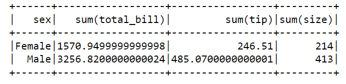

We can apply .groupBy( ) and .select( ) methods together. Here is an example where we calculated the day wise maximum tip.

### Group by day, max tip
df_pyspark.groupBy("day").max().select(["day", "max(tip)"]).show()

We can also apply .count( ) method to count number of observations for each day label/categories.

df_pyspark.groupBy("day").count().show()

We can achieve similar result by supplying the column as key and functionality as value inside a dictionary.

df_pyspark.agg({"tip": "sum"}).show()

Here is an example where we have calculated the sum of tip and maximum of total_bill for each gender label/category.

df_pyspark.groupBy("sex").agg({"tip": "sum", "total_bill": "max"}).show()

Finally, close the spark session once you’re done with it using the .stop( ) method.

spark.stop()

PySpark is one of the best tools available to deal with Big data. For python users, it is straightforward to learn and implement due to the similarity with pandas + SQL functionalities. I hope this article gives you motivation to apply it in your work.

Click here for thedata and code

I hope you’ve found this article useful!