Rahul Raoniar
- posted on
- Comments Off on How to use Stata and Python Together Directly from Jupyter Notebook
Introduction
Stata is a popular data analytics tool used by researchers for statistical analysis. Nowadays, there are numerous tools available for performing data analysis. The popular open-source programming tools like R and Python. Even though R and Python are open source and easy to implement, they are still not mature. What I felt after learning R and Python is that R has numerous libraries, but the syntax are not consistent across libraries, which sometimes makes it hard for research work. In case of python, the syntax are consistent but many statistical analysis methods or modelling approach are still not available or are in the phase of development. Thus, I have to often depend on paid software products which are feature rich and mature. Stata is one of them that I often use for research related analysis. Now Stata 17 offers integration with Python which makes the analysis process super easy and fun.
Let’s say you are doing some analysis in python and want to do some statistical analysis. You searched the internet and realized that the implementation of the statistical model is not available in Python, or not the exact implementation available that you want, then you have to approach a paid software and perform the analysis.
Stata’s new Jupyter notebook support makes it super easy. Now, you can send data from python to Stata and vice versa. For example, you can send a part of the data from python to Stata, conduct analysis and return the output to Python for further analysis or vice versa. This can be done entirely from Jupyter notebook.
Aim of the Article
The aim of the article is to illustrate how we could utilise Python and Stata together to perform statistical analysis directly from Jupyter notebook.
Article Outline
- Stata in Ipython Notebook
- Loading a Dataset Into Python and Transferring it to Stata for Analysis
- Transferring Predictions from Stata to Python
1. Stata in Ipython Notebook
Loading Stata
To use the Stata in Ipython Notebook. First, you need to set up Python. Here, I’m using anaconda distribution and Python version 3.7. You need to ensure that you have Stata 17, which provides integration of Stata and Python in Ipython notebook/ Jupyter Notebook.
To start with the Ipython notebook you need to install stata-setup package/library using pip.
pip install stata-setup
Next, open an Ipython notebook, and you need to import stata_setup module. Further, we need to use stata_setup.config( ) and supply the directory where the Stata exist in your local machine, also specify the edition of Stata. Here in my case I’m using the Basic Edition so, “be”.
Once you run it, you will see the following Stata page, indicating you are now connected to Stata desktop.
import stata_setup
stata_setup.config("D:\Application Installation\STATA", "be")
Load auto Data in Stata
First, I’m going to set the white tableau scheme permanently, which is a wonderful plot scheme.
You can enable it by installing schemepack package developed by Asjad Naqvi. Follow the link for installation instructions: Link.
In jupyter notebook, to send any instruction to Stata we need to initiate the command with a %%stata magic command.
%%stata
set scheme white_tableau, perm
Once, we set the tableau scheme; next we start analysing data. Let’s load the auto data.
Here, we used the system default auto data and summarize it.
%%stata
sysuse auto, clear
summarize
Generating a Scatter Plot
Let’s generate a scatter plot between mpg and weight for Domestic and Foreign cars separately using the twoway command.
%%stata
twoway (scatter mpg weight, msize(vlarge)), by(foreign)
2. Loading a DataSet Into Python and Transferring it to Stata for Analysis
Let’s load the inbuilt tips data from Python’s Seaborn library.
import seaborn as sns
tips = sns.load_dataset("tips")
tips.head()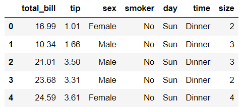
We can also check the value counts for categorical data.
tips["time"].value_counts()
Before we send this data to Stata we need to ensure that there are no other data in Stata memory. Thus, it is good practice to clear the memory using clear command.
%%stata
clear
Transferring Data from Python to Stata
To transfer the tips data to Stata we need to use -d datasetname
We can now use list in 1/5 to print top five observations
%%stata -d tips
list in 1/5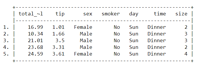
Let’s summarize the data using summarize command. It only produced summary for the continuous data, i.e., total_bill, tip and size.
%%stata
summarize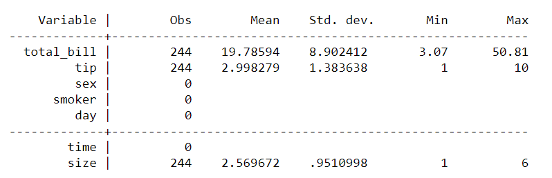
Let’s see the data format/type using the describe command.
%%stata
describe
You can observe that sex, smoker, day and time are in string format.The next step is to encode the labels and transform them into categorical variables (sex, smoker, day and time).
Label sex
We label the sex → 0: Male and 1: Female and save it into another variable called sex_enc.
%%stata
label define sex_lab 0 "Male" 1 "Female"
encode sex, gen(sex_enc) label(sex_lab)
tab sex_enc
Label smoker
We label the smoker status → 0: No and 1: Yes and save it into another variable called smoker_enc.
%%stata
label define smoker 0 "No" 1 "Yes"
encode smoker, gen(smoker_enc) label(smoker)
tab smoker_enc
Label time
We label the time → 0: Lunch and 1: Dinner and save it into another variable called time_enc.
%%stata
label define time_lab 0 "Lunch" 1 "Dinner"
encode time, gen(time_enc) label(time_lab)
tab time_enc
Label Day
We label the Day status → 0: Sat, 1: Sun, 2: Thur and 3: Fri and save it into another variable called day_enc.
%%stata
label define day_lab 0 "Sat" 1 "Sun" 2 "Thur" 3 "Fri"
encode day, gen(day_enc) label(day_lab)
tab day_enc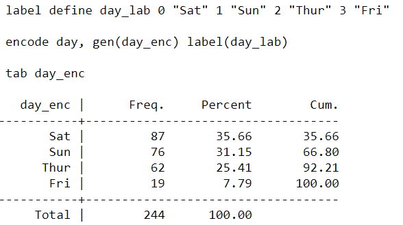
Chi-square Test of Independence
Once we label all categorical variables, let’s check whether the categorical variables are acting as it should act in Stata. Let’s conduct a Chi-square test of independence and check whether sex and smoker are related. The test statistics (p>0.05) revealed that sex and smoker are independent.
%%stata
tab sex_enc smoker_enc, chi2
Fit a Linear Regression Model
Let’s fit a linear regression using reg Stata command. It worked as expected.
%%stata
reg tip total_bill ib(0).smoker_enc ib(0).sex_enc ib(0).time_enc ib(0).day_enc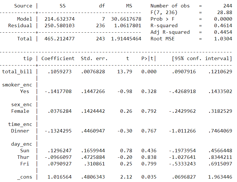
Compute margins
Let’s generate a margin plot by supplying the total bill from 3 to 50 at an interval of 5, while holding other variables constant.
%%stata
quietly margins, at(total_bill=(3(5)50))
marginsplot
3. Transferring Predictions from Stata to Python
Sometimes we may need to transfer some estimates from Stata to Python to perform any computation on that. Say, we want to transfer the margin estimate computed previously to Python. We can use the -doutd and save it to preddata. We will use this preddata in next step.
For now, let’s calculate the margin again and save it in Stata as predictions. Now, if we print the predictions, we can see the name of the columns total_bill as _at1 and margins as _margin. Let’s rename the columns as total_bill and pr_tip.
%%stata -doutd preddata
quietly margins, at(total_bill=(3(5)50)) saving(predictions, replace)
use predictions, clear
list _at1 _margin in 1/5
rename _at1 total_bill
rename _margin pr_tip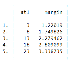
If we now access the two columns from preddata and print the first 5 observations in Ipython notebook. It will print the data as pandas dataframe.
preddata[['total_bill', 'pr_tip']].head()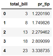
Stata is a wonderful software for performing statistical analysis. Similarly, Python is a wonderful general purpose programming language. We can use both of them parallelly to harness the power to solve both statistical and machine learning related problems.
Click here for the data and code
I hope you’ve found this article useful!