One Zero Blog

Article Outline

• Aim of the article
• About Dataset
• Loading Libraries and Data
• Descriptive Statistics
• Grid Search based Hyperparameters Tuning
• Random Grid Search based Hyperparameters Tuning
• Genetic Algorithm based Hyperparameters Tuning
• Code and Data

Aim of the article

The aim of the article is to predict concretes characteristics compressing strength (regression problem) using Gradient Boosting Machine (GBM) and tune its hyperparameters to reduce model overfitting.

About Dataset

I have a Transportation Engineering (Civil Engineering Domain) background. During my civil engineering Diploma, B.Tech and M.Tech I had performed the Concrete’s Characteristics Compressive Strength test in a laboratory setting. Thus, I thought it would be interesting to model the concrete’s compressive strength using a tree-based ensemble (Gradient Boosted Regressor).

Hence, in this article, we are going to use the concrete dataset [1] obtained from the UCI Machine Learning library.

The dataset includes the following variables, which are the ingredients for making durable high strength concrete.

I1: Cement (C1): kg in a m3 mixture
I2: Blast Furnace Slag (C2): kg in a m3 mixture
I3: Fly Ash (C3): kg in a m3 mixture
I4: Water (C4): kg in a m3 mixture
I5: Superplasticizer (C5): kg in a m3 mixture
I6: Coarse Aggregate (C6): kg in a m3 mixture
I7: Fine Aggregate (C7): kg in a m3 mixture
I8: Age: Day (1~365)
O1: Concrete compressive strength: MPa

Where I: Input; O: Output, C: Component; m3: meter cube and MPa: Megapascal.

Before proceeding to the data analysis part, let’s get familiar with the different inputs of the concrete dataset.

Concrete

Concrete is comprised of three basic components: water, aggregate (rock, sand, or gravel) and cement. Cement acts as a binding agent when mixed with water and aggregates.

Compressive Strength

Compressive strength is one of the vital parameters that determine the performance as a construction material. A concrete mix designed to get the required performance and durability for a given construction work/project. The compressive strength of concrete is determined in laboratories in order to maintain the desired quality of concrete during casting. The compressive strength is calculated by dividing the failure load with the area of application of load, usually after 28 days (I8: Age) of the curing period. Though researchers also report strength after 7, 14 and 21 days of curing period. The strength of concrete is achieved by controlling the proportion of cement (C1), fine (C7) and coarse (C6) aggregates, water, and various admixtures. The characteristic compressive strength of concrete fc/ fck is usually reported in MPa (O1). For normal Construction, the characteristic compressive strength can vary from 10 to 60 MPa; while for a certain structure the requirement can go beyond 600 MPa.

Admixture

Nowadays, researchers are using different admixtures to get desired property; the fly ash (C3) is one of them. The fly ash act as an admixture in concrete mixes, which is a pozzolan substance containing aluminous and siliceous material; when mixed with lime and water, forms a compound similar to cement. Fly ash is mixed in concrete as an admixture to improve workability and to reduce permeability and bleeding.

Similarly, the ground granulated blast furnace slag (C2), a mineral admixture is added in concrete to improves its properties such as workability, strength and durability.

Superplasticizers

Superplasticizers (high range water reducers) are used in concrete mixes for making high strength durable concrete. Superplasticizers (C5) are water-soluble organic substances that reduce the amount of water require to achieve certain stability of concrete, reduce the water-cement ratio, reduce cement content and increase slump. Use of superplasticizers reduces the water requirement up to 30% without losing workability.

Loading libraries

The very first step is to install and load the following libraries.

import pandas as pd    # Data manipulation
import numpy as np     # Array manipulation

# GBM regressor
from sklearn.ensemble import GradientBoostingRegressor

# Train Test Split
from sklearn.model_selection import train_test_split

# Data Preprocessing (Scaling)
from sklearn.preprocessing import StandardScaler

# Model Evaluation
from sklearn.metrics import mean_absolute_error

# Grid and Random CV Search
from sklearn.model_selection import GridSearchCV, RandomizedSearchCV

# Genetic Algorithm based Search
from tpot import TPOTRegressor

Loading data

The next step is to load the data from an excel sheet from your local storage and performing basic exploratory data analysis.

concrete = pd.read_excel("Concrete.xlsx")
concrete.head()

Let’s view the different column names using .column attribute.

concrete.columns

The next step is to check the number of observations, variables and column types. The dataset contains 1030 observations and 9 columns. The data consist of floats and integers.

concrete.info()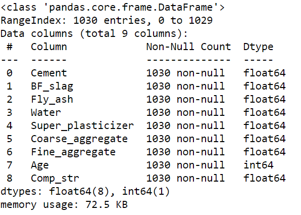

In order to check the basic descriptive statistics, one can use the .describe attribute.

concrete.describe()

Let’s assign the X variables (independent variables) after dropping the “Comp_str” and Y variable (outcome variable: Comp_str). We can check the shape of the X and y using .shape attribute.

X = concrete.drop("Comp_str", axis = 1)
y = concrete["Comp_str"]
print(X.shape)
print(y.shape)

The next step is to split the data into train and test. As the dataset is small so we are not going to make a separate validation set here. We can split the data set into 80% train and 20% test using the train_test_split( ) method. Additionally, for reproducibility, we are setting a random_state.

X_train, X_test, y_train, y_test = train_test_split(X, y, test_size = 0.20, random_state = 42)

Before training, it is a good idea to scale the variables so that the algorithms optimize the learning process faster. Here, we are going to use the StandatdScaler( ) method from sklearn.model_selection class. First, we initialize the StandardScaler( ) object and apply fit_transform( ) method only on train data (not test). Then we use the scaler object to only transform the test dataset. This is because we do not want to show the test data to our model during the training process i.e., we keep the test data separate and use it only for testing.

scaler = StandardScaler()
X_train_scaled = scaler.fit_transform(X_train)
X_test_scaled = scaler.transform(X_test)

Grid Search

Before we proceed for model training and hyperparameters tuning, it is a good idea to check what type of parameters it offers. We can check this by first initializing the model object GradientBoostingRegressor(criterion = “mae”) then applying the .get_params() method. It is also recommended to read some blog or research paper to identify the best parameters which you could tune to improve the model performance. Here, we are going to use Mean Absolute Error (MAE) as a model evaluation metric (lower value represents better fit) as it is less sensitive to outliers in data set.

clf = GradientBoostingRegressor(criterion = "mae")
clf.get_params()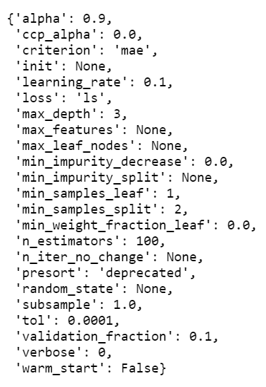

Here, based on past research I have opted for max_depth, n_estimators, max_features, and criterion hyperparameters to tune our model. The hyperparameters have the following definition.

max_depth: Maximum depth of a tree.

n_estimators:the number of trees which needs to be built before taking an average of predictions.

max_features:The number of features to consider when looking for the best split.

criterion: The function to measure the quality of a split.

In the tuning process, one of the gold standards is to use cross-validation and taking the average result which provides reliable estimates of model performance. Here, we first perform a grid search of all combinations of hyperparameters. The parameters are added as a key-value combination inside a dictionary (param_grid). To try multiple values of hyperparameters we need to supply it as a list.

In order to start training, you need to initialize the GridSearchCV( ) method by supplying the estimator (gb_regressor), parameter grid (param_grid), a scoring function; here we are using negative mean absolute error as we want to minimize it. Then we set n_jobs = 4 to utilize 4 cores of the system (PC or cloud) for faster training. GBM training also supports GPU. Here, we are going to fit a 10-fold cross-validation model. Further, enabling refit=True refit the model with the best hyperparameters once tuning finished.

# Create a Gradient Boosted Regressor with specified criterion
gb_regressor = GradientBoostingRegressor(criterion = "mae")

# Create the parameter grid
param_grid = {'max_depth' : [2, 4, 8, 10, 12],
              'n_estimators' : [100, 200, 300],
              'max_features' : ['auto', 'sqrt'],
              "criterion" : ["friedman_mse", "mse", "mae"]}

# Create a GridSearchCV object
grid_gb = GridSearchCV(
    estimator = gb_regressor,
    param_grid = param_grid,
    scoring = 'neg_mean_absolute_error',
    n_jobs = 4,
    cv = 10,
    refit = True,
    return_train_score = True)
print(grid_gb)

The next step is to call the fit( ) method over the CV object (grid_gb) with scaled train data to start model training.

grid_gb.fit(X_train_scaled, y_train)

Once the model training start, keep patience as Grid search is computationally expensive and takes time to complete.

Once the training is over, you can access the best hyperparameters using the .best_params_ attribute. Here, we can see that with a max depth of 4 and 300 trees we could achieve a good model.

grid_gb.best_params_

Let’s see the score. The model with tuned hyperparameters (best parameters) provides an average neg mean absolute error of 2.91 which is really good.

One thing to note that, the actual MAE is simply the positive version of the number we’re getting.

The unified scoring API always maximizes the score, so scores which need to be minimized are negated in order for the unified scoring API to work correctly. The score that is returned is therefore negated when it is a score that should be minimized and left positive if it is a score that should be maximized. You can read more about this here.

grid_gb.best_score_

We can also convert the CV results to a data frame and identify the row which includes the best CV parameters.

cv_results = pd.DataFrame(grid_gb.cv_results_)

# Extract and print the row that had the best mean test score
best_row = cv_results[cv_results['rank_test_score'] == 1]
print(best_row)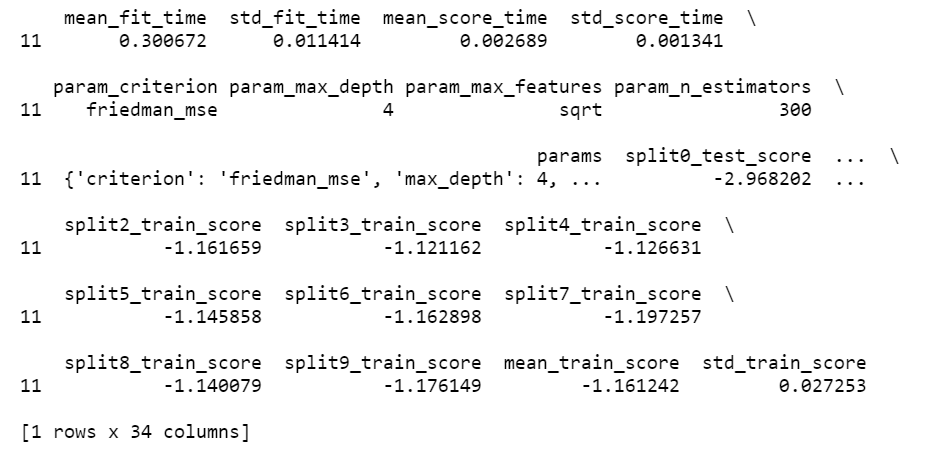

We can also able to access different parts of the result by indexing it from best parameters. Here, I have extracted the number of estimators used by the best-fitted model, which is 300.

grid_gb.best_params_["n_estimators"]

The next vital step is to check how your model will generalize on unseen or test data. That is the ultimate test for your tuned model. From the tuned model object we could grab the best estimator and use the predict( ) method to predict the scaled test dataset. As during the training process, we kept the argument refit = True thus, even if you apply the predict( ) method on trained CV object, it will directly fetch the best-tuned estimator for prediction.

Here, we can observe that the MAE for test prediction is 2.86 which is overall good and near to the CV results (2.91), indicating no/negligible overfitting.

predictions = grid_gb.best_estimator_.predict(X_test_scaled)
mean_absolute_error(predictions, y_test)

Random Grid Search

Next, we will dive into a world where we need less computation. Welcome to the world of random search. The past studies highlighted that random search could be a more efficient way of model training which reduces the time required for getting an optimal solution [2]. The modelling process is the same as we did before for GridsearchCV( ), the only difference is that you now need to initialize the CV with a RandomizedSearchCV( ) method.

# Create a Gradient Boosted regressor with specified criterion
gb_regressor = GradientBoostingRegressor(criterion = "mae"
)

# Create the parameter grid
param_grid = {'max_depth' : [2, 4, 8, 10, 12],
              'n_estimators' : [100, 200, 300],
              'max_features' : ['auto', 'sqrt'],
              "criterion" : ["friedman_mse", "mse", "mae"]}

# Create a Randomized Search CV object
random_grid_gb = RandomizedSearchCV(
    estimator = gb_regressor,
    param_distributions = param_grid,
    scoring = 'neg_mean_absolute_error',
    n_jobs = 4,
    cv = 10,
    refit = True,
    return_train_score = True)
print(random_grid_gb)

Next, we fit the data using .fit( ) method.

random_grid_gb.fit(X_train_scaled, y_train)

We can retrieve the best hyperparameters using the .best_params_ attribute.

random_grid_gb.best_params_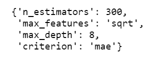

The average 10-fold CV score is 2.99

random_grid_gb.best_score_

The prediction on the test data showed an MAE of 2.99, indicating an overall good performance on the test dataset.

Genetic Algorithm based Search

Genetic algorithm is related to the world of biology, specifically the field of genetics. The genetic algorithm works as similar to living creatures’ genetic evaluation in the real world. The concept states that in the world many creatures exist and the strongest among them pair off. There are crossovers where they form offspring and there are random mutate exist in the crossover process. This random crossover provides some advantages to some offspring and the cycle continues.

The same concept has been utilized by researchers for developing the genetic algorithm. Now, researchers and data scientists are using the same algorithm for machine learning model hyperparameters tuning.

The process involved the following steps:

i) We fit several models with hyperparameters

ii) We pick the best out of them (those who survived/ strong)

iii) Then we create models (offspring) which are similar to the best ones (strong ones)

iv) We add randomness to it so that we could avoid local minima

v) We repeat the process until we get the best one

Here, in this example, we are going to use a library called tpot that provides a fast implementation of genetic-based model hyperparameters search.

As this is a regression problem, thus we will import the TPOTRegressor from tpot library.

from tpot import TPOTRegressor

Next, we initialize the parameters such as number_generations, population_size, offspring_size and scoring_function.

generations: Number of iterations to run the optimization process.
population_size: Number of models to keep after each iteration
offspring_size: Number of models to produce in each genetic programming iteration.

Here, we are fitting the model with the 10-fold CV, using the “negative mean absolute error” scoring function.

# Assign the inputs
number_generations = 20
population_size = 10
offspring_size = 10
scoring_function = 'neg_mean_absolute_error'

# Create the tpot regressor
tpot_reg = TPOTRegressor(generations = number_generations,
                         population_size = population_size,
                         offspring_size = offspring_size,
                         scoring = scoring_function,
                         verbosity = 2,
                         random_state = 2,
                         cv = 10,
                         n_jobs = -1)

Next, we fit the model to the data and evaluate the score. The below figure illustrated that the optimization process is complete. 

# Fit the regressor to the training data
tpot_reg.fit(X_train_scaled, y_train)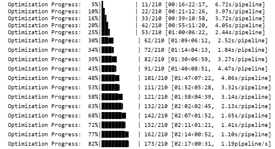

At the end of the training, it also highlights the best hyperparameters and modelling algorithm to use for gaining an accurate solution. Here, it revealed that XGBoost Regressor could be the best candidate for this data. 

Best pipeline: XGBRegressor(MinMaxScaler(input_matrix), learning_rate=0.1, max_depth=8, min_child_weight=4, n_estimators=100, nthread=1, objective=reg:squarederror, subsample=0.6000000000000001)

The model evaluation on the test dataset showed an MAE of 2.85, indicating an overall good performance on the test dataset.

# Score on the test set
print(tpot_reg.score(X_test_scaled, y_test))

-2.8526538220688846

You can use large number_generations, population_size and offspring_size to find a good model.

I hope you learned something new!

Code and Data

References

[1] I-Cheng Yeh, “Modeling of the strength of high-performance concrete using artificial neural networks,” Cement and Concrete Research, Vol. 28, №12, pp. 1797–1808 (1998).

[2] Bergstra J., & Bengia, Y. (2012). Random Search for Hyper-Parameter Optimization. Journal of Machine Learning Research, 13, 281–305.

Featured image credit: Photo by Anthony Martino on Unsplash