One Zero Blog

Introduction

Survival analysis is a branch of statistics for analysing the expected duration of time until one or more events occur. The method is also known as duration analysis or duration modelling, time-to-event analysis, reliability analysis and event history analysis.

The survival analysis is used to analyse following questions:

• A proportion of population surviving up to a given time
• Rate at which they are dying
• Understanding the impact of covariates on survival

The survival analysis is used in various field of research:

• Medical: Understanding patient’s survival when diagnosed with a deadly disease
• Medical: Hospital readmission duration after a major heart surgery
• Industry: When would Tesla car battery permanently die/fail
• Transportation: Waiting time of pedestrian after red (do-not walk) phase arrival at intersection
• E-commerce: After seeing ads when a person would purchase the product
• Human resource: When an employee would leave a company (churn)

There are various methods used by researchers to understand the time to event analysis. In this article, we are going to learn, the following types of models and try to understand their mechanism in time to event analysis.

• Kaplan-Maier Estimate (Non-parametric)
• Cox Proportional Hazard Model (Semi-parametric)
• Accelerated Failure Time Model (Parametric)

Aim of the Article

The aim of the article is to understand the survival of lung cancer patents using time to event analysis.

Note: If you are not familiar with the survival analysis, then I will highly recommend reading some articles and watching some YouTube videos on survival analysis. Here are a few reading and video resources to learn about survival analysis:

Reading Resources
Blog 1: Link
Blog 2: Link

Video Resources
Survival analysis concept videos
1. Channel: MarinStatsLectures-R Programming & Statistics: Link
2. Channel Zedstatistics: Link

• The current article presented an implementation of time to event analysis using Stata 17 software.

Article Outline

• Description of lung cancer data
• Imputing missing values
• Kaplan Meier curve estimation
• Fitting Cox Proportional Hazard Regression
• Cox model results interpretation
• Testing Proportional Hazard assumption
• Fitting Accelerated Failure Time (AFT) Model
• AFT model results interpretation

Let’s start !!!!!!

Lung Cancer Data

First, we need to know about the lung cancer data that we are going to use for the analysis. The data is originally available in R programming language (in survival library) [1]. So, I have downloaded it from R to use it for learning purpose. The data source is mentioned below.

Data Source: Loprinzi CL. Laurie JA. Wieand HS. Krook JE. Novotny PJ. Kugler JW. Bartel J. Law M. Bateman M. Klatt NE. et al. Prospective evaluation of prognostic variables from patient-completed questionnaires. North Central Cancer Treatment Group. Journal of Clinical Oncology. 12(3):601–7, 1994.

Data Description

The data consist of 228 observations and 10 variables/columns. The variable description is presented as follows:

• inst: Institution code
• time (d1): Survival time in days
• status (d2): censoring status 1 = censored, 2 = dead
• age (i1): Age in years
• sex (i2): Male = 1 Female = 2
• ph.ecog (i3): ECOG performance score as rated by the physician. 0 = asymptomatic, 1 = symptomatic but completely ambulatory, 2 = in bed <50% of the day, 3 = in bed > 50% of the day but not bed bound, 4 = bed bound
• ph.karno (i4): Karnofsky performance score (bad = 0; good = 100) rated by physician
• pat.karno (i4): Karnofsky performance score as rated by patient
• meal.cal (i5): Calories consumed at meals
• wt.loss (i6): Weight loss in last six months

Where: ‘i’ indicates the independent variables (covariates), and ‘d’ indicates dependent variables. Actually, the dependent variable or response is the time until the occurrence of an event (i.e., the lung cancer patient dies).

Reading Data into Stata

First, let’s read the lung.csv data from our local storage.

step1.: fix the current working directory using ‘cd’

step2: using import command, load the data into Stata

The data contains 228 observations and 10 variables/columns.

clear
cd "set path of your working directory"
import delimited "lung.csv"

The next step is to check the data description and data types using describe command. The variables in the dataset are either integer or byte type.

describe

Adding Labels/Description of Variables

In the next step, we will add labels to the variables that helps us to recall the meaning of the coded variables. It is very helpful, if we need to visit the data in future.

To label a variable, we need to use label variable command then supply the column name and label string in quotation mark (‘‘ ’’). Now describe command displays the variable labels in the “variable label” column.

label variable inst "Institute code"
label variable time  "Survival time in days"
label variable status "censoring status 1 = censored, 2 = dead"
label variable age "Age in years"
label variable sex "Male = 1 Female = 2"
label variable ph_ecog "ECOG performance score as rated by the physician. 0 = asymptomatic, 1 = symptomatic but completely ambulatory, 2 = in bed <50% of the day, 3 = in bed > 50% of the day but not bedbound, 4 = bedbound"
label variable ph_karno "Karnofsky performance score (bad=0-good=100) rated by physician"
label variable pat_karno "Karnofsky performance score as rated by patient"
label variable meal_cal "Calories consumed at meals"
label variable wt_loss "Weight loss in last six months"
describe

Checking Missing Values

The next step will be to check for missing values in the variables. In Stata, we can use a user-defined library/package to count the missing values. The mdesc package can be installed by searching the package name. After installation, we can run the mdesc command, which creates a table for missing value counts and its proportion in separate columns.

The resulting table illustrates the following:

inst: 1 missing value
ph.ecog: 1 missing value
ph.karno: 1 missing value
pat karno: 3 missing values
meal.cal: 47 missing values
wt.loss: 14 missing values

//search mdesc package and install it
mdesc

Let’s check the label count in ph.ecog categorical column. This variable has one missing value and the label count shows that label 3 has only one observation that we should remove from the model, as it won’t make much contribution to the model.

tab ph_ecog

The next step is to remove the missing value and label 3 from ph_ecog variable. Additionally, I have imputed the ph_karno, pat_karno, meal_cal and wt_loss with their mean value using a for loop, as I don’t want to lose more sample and this analysis part is only for demonstration purpose.

If we now run the mdesc command, we can observe that there is no missing value in the variables. Only inst variable has 1 missing value, and we can keep it like that as we are not going to use this variable in our model.

drop if ph_ecog == .
drop if ph_ecog == 3
for var ph_karno pat_karno meal_cal wt_loss: 
  summ X \\ replace X = r(mean) if missing(X)

mdesc

Labelling Values of Categorical Columns

The next step is to label values for the categorical variables using the following steps:

• define a labelling scheme
• applying the label to the categorical variable

Here, we have labelled status, sex and ph_ecog categorical variables.

label define statuslab 1 "censored" 2 "dead"
label values status statuslab
label define genderlab 1 "Male" 2 "Female"
label values sex genderlab
label define ecoglab 0 "asymptomatic" 1 "symptomatic" 2 "in_bed<50" 
label values ph_ecog ecoglab

Saving Final Dataset in Stata (filename.dta format)

Now, the preprocessing of the data is complete, and we can save this data in Stata (.dta) format using save command.

Next, we can directly import the “Survival analysis of lung data stata.dta” file directly using the use command. Now, everything looks good, so we can proceed with the analysis.

//Save and use data
save "Survival analysis of lung data stata.dta" , replace
clear
cls
use "Survival analysis of lung data stata"
describe

Descriptive Statistics

Let’s check the descriptive statistics of the data using summarize (su) command. The command generates descriptive statistics only for continuous data.

summarize time age ph_karno pat_karno meal_cal wt_loss

Distribution of Time Variable

Let’s, plot a histogram (using histogram command) of the time variable to get an overall idea of the distribution. The histogram shows that the time variable almost follows a Weibull or Log-normal distribution. We will check that during the AFT model estimation part.

histogram time, width(25) frequency fcolor(eltblue) lcolor(black%70) lwidth(vthin) kdensity kdenopts(lcolor(orange_red)) xtitle(Time in days)

Declaring Data to be Survival-Time Data

Before we proceed with the survival analysis models, we need to declare the time and failure event (status) variables using stset command.

stset time, failure(status == 2)

Kaplan-Maier Curve Fitting (Non-Parametric Model)

To start with survival analysis, the first step is to plot a survival curve of the overall data. It can be done by generating a Kaplan-Maier curve.

The Kaplan-Meier approach, also called the product-limit approach, is a popular approach which re-estimates the survival probability each time an event occurs. It is a non-parametric method, means it does not assume the distribution of the outcome variable (i.e., time).

We can use the sts graph command to generate a K-M plot. We can also supply the risktable command that generates a risk table underneath the plot.

The curve illustrates how the survival probabilities change over the time horizon. As the time passes, the survival probabilities of lung cancer patents decreases.

sts graph, risktable ylabel(, format(%9.1f))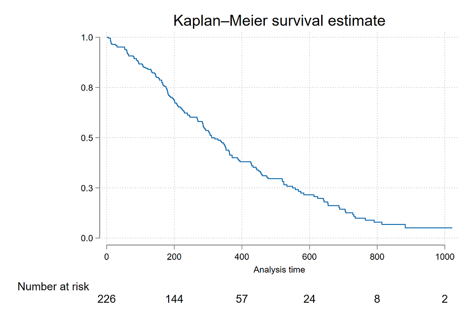

K-M Plot by Gender/Sex Categories

Using the K-M estimate, we can check the difference between categorical groups. Though, it is only viable when the variable has fewer categories. Here is an example where we are plotting the two survival curves, one for Male and another for Female.

The command is the same only we need to add a by(sex) option, which split the data by gender, i.e., Male and Female and generate two separate K-M plots.

The curve illustrates that the survival probabilities of female patients are overall higher compared to male patients at any instance of time.

sts graph, by(sex) risktable ylabel(, format(%9.1f))

Cox-Proportional Hazard Model (Semi-Parametric Model)

Cox-PH model is a semi-parametric model which solves the problem of incorporating covariates. In Cox’s proportional hazard model, the log-hazard is a linear function of the covariates and a population-level baseline hazard [2].

In the above equation, the first term is the baseline hazard and the second term known as partial hazard. The partial hazard inflates or deflates the baseline hazard based on covariates.

Cox-PH Model Assumptions

Cox proportional hazards regression model assumptions include:

• Independence of survival times between distinct individuals in the sample
• A multiplicative relationship between the predictors and the hazard, and
• A constant hazard ratio over time

Definition of Hazard and Hazard Ratio

• Hazard is defined as the slope of the survival curve. It is a measure of how rapidly subjects are dying.
• The hazard ratio compares two groups. If the hazard ratio is 2.0, then the rate of deaths in one group is twice the rate in the other group.

Fitting Cox-PH Model

To fit the Cox Proportional Hazard model, we need to use the stcox command and then supply the independent variables. The categorical columns were added with their base value indicator [ib(category)]. I have added the allbaselevels option to print the base labels in the summary table.

The summary table provides coefficients, standard error, z statistics, p-values and confidence intervals.

Note: To display the coefficients instead of hazard ratios, we need to add nohr option in the command.

stcox age ib(1).sex ib(0).ph_ecog ph_karno pat_karno meal_cal wt_loss, allbaselevels nohr cformat(%9.3f) pformat(%5.3f) sformat(%8.3f)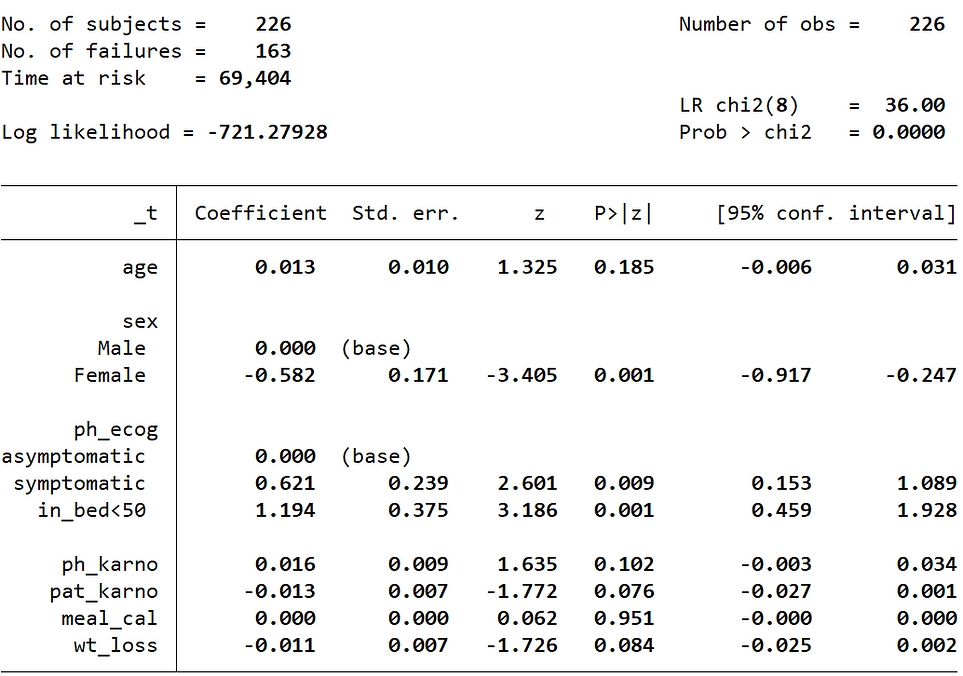

Cox-PH Estimates with Hazard Ratios

If we do not supply the nohr option, then it will print the same table but with a hazard ratio column.

stcox age ib(1).sex ib(0).ph_ecog ph_karno pat_karno meal_cal wt_loss, allbaselevels cformat(%9.3f) pformat(%5.3f) sformat(%8.3f)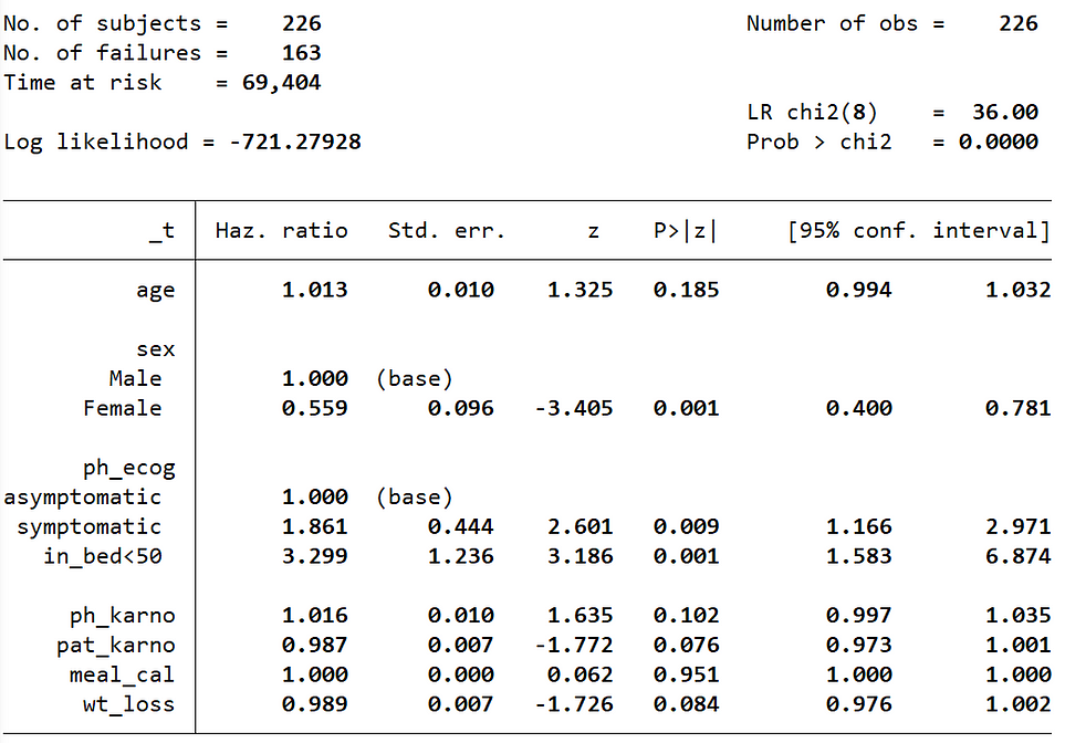

Interpretation of Cox-PH Model Results/Estimates

The interpretation of the model estimates will be like this:

• Wt_loss has a coefficient of about -0.011
• We can recall that in the Cox proportional hazard model, a higher hazard means more at risk of the event occurring
• The value exp(-0.011) is called the hazard ratio
• Here, a one unit increase in the weight loss means the baseline hazard will increase by a factor of exp(-0.011) = 0.99 -> about a 1% decrease
• Similarly, the values in the ecog column are: [0 = asymptomatic (base), 1 = symptomatic but completely ambulatory, 2 = in bed <50% of the day]. The value of the exponentiated coefficient associated with ecog2 (in bed <50% of the day) i.e., exp(1.194), is the value of ratio of hazards associated with being “in bed <50% of the day (coded as 2)” compared to asymptomatic (coded as 0; base category). This indicates the risk (rate) of dying is 3.299 times for patients who are “in bed <50% of the day” compared to asymptomatic patients.

Post Estimation

After model fitting, the next step is to check the model fit statistics. We can use the estat ic command to estimate Akaike Information Criterion (AIC) and Bayesian Information Criterion (BIC) statistics.

estat ic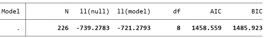

Concordance Index

Concordance index or C-index is used to evaluate the model predictions. It ranges from 0.5 to 1. The C-index of 0.5 indicates a poor performing model, while a value of 1 indicates a model with perfect prediction. We can estimate C-index using the estat concordance command. The estimate table shows that the Harrell’s C value is around 0.65.

estat concordance

Plotting Cox PH Survivor or Related Functions

Next, we could check the fitted model’s overall survival, hazard, and failure over time using different plots.

Survival Function of Cox Model

The first plot and most basic one is generating survival plot of the Cox-PH model using stcurve, survival command.

stcurve, survival ylabel(, format(%9.1f))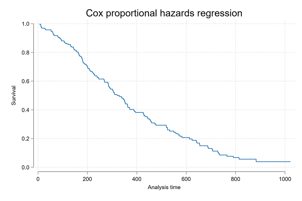

Survival Functions of Cox Model Over Gender Categories

We can plot separate survival curves for categorical groups. For example, here we have plotted two separate survival curves; one for Male and another for Female patients by supplying an additional group option at(sex = (1 2)).

stcurve, survival at(sex = (1 2)) ylabel(, format(%9.1f))

Hazard Function of Cox Model

Instead of survival, if we supply the hazard in the option, it will generate a hazard curve.

stcurve, hazard

Cumulative Hazard Function of Cox Model

We can generate a cumulative hazard curve by supplying the cumhaz in the command option.

stcurve, cumhaz ylabel(, format(%9.1f))

Failure Function of Cox Model

To generate a failure plot (opposite of survival plot) you need to supply the failure argument.

stcurve, failure ylabel(, format(%9.1f))

Cox’s Proportional Hazard Assumption Test

Once we fit the model, the next step is to verify the proportional hazard assumption.

The null (H0) hypothesis assumed that the proportional hazard criteria satisfied, while alternative hypothesis (H1) infer that the proportional hazard assumption criteria not met (violated).

We can directly use the estat phtest command and also supply the detail command to generate test statistics table.

The result revealed that at 5% significance level, ph_karno and meal_cal violated the assumption. The global p-value also indicates that the assumption is violated. There are various approach to deal with it, for example we can convert meal_cal to a binned category, or we can use a parametric Cox-PH model.

estat phtest, detail

Log-Log Plot for Gender (Cox PH Test)

A visual way of checking the assumption is by generating a log-log plot. If the plotted categories are parallel and don’t cross each other, then we can assume that the selected categorical variable satisfied the assumption. For example, here, gender categories are almost parallel thus, satisfied the PH assumption.

stphplot, by(sex) ylabel(, format(%9.1f))

Log-Log Plot for ph_ecog

If we check the log-log plot for ph_ecog we can see that the lines crossed each other which implies violation of the assumption.

stphplot, by(ph_ecog) ylabel(, format(%9.1f))

Accelerated Failure Time Model (Parametric Model)

If the proportional hazard assumption criteria of Cox-PH model is not satisfied, in such instance, a better approach is to use a parametric model. Accelerated Failure Time (AFT) is one of the popular parametric model used in survival analysis.

The model assumes that the survival function follows a parametric continuous distribution. For instance, one can assume a Weibull distribution or a Log-normal distribution.

The parametric AFT model assumes that survival function that derived from say two population (for example P and Q) are related by some acceleration factor lambda (λ), which can be modelled as a function of covariates.

Based on the covariates, the AFT model can accelerate or decelerate the failure times. The AFT model coefficients can be interpreted easily: a unit increase in a covariate means the average/median survival time changes by a factor of exp(b_i) [2].

Identifying the Best Fitted Distribution

There are many distributions exist that we can fit. So, the first step is to identify the best distribution that best fits the data. The common distributions are Weibull, Exponential, Log-Normal, Log-Logistic and Generalized Gamma.

Here is a step-by-step guide for identifying best fitted distribution:

• First create a frame called ics with three columns the model name, aic and bic.
• Declare model as str32, and aic and bic as float
• Use a for loop to iterate over different distribution name and fit a model to generate fit statistics
• Store the model name and fit statistics (AIC and BIC) into the earlier defined frame called ics
• Change the current frame to ics and list the sorted observations (based on ascending order of aic and bic values)
• Once inspection work is done with ics frame, then we need to return to the default frame i.e, our refined version of the lung cancer data

The model with the lowest AIC and BIC values is the best fitted model. Here, Weibull [aic: 535.55; bic: 569.75] is the best fitted model. So, we can proceed with Weibull distribution.

frame create ics str32 model float(aic bic)
foreach model in exponential loglogistic  weibull lognormal ggamma  {
    quietly streg age ib(1).sex ib(0).ph_ecog  ph_karno pat_karno meal_cal wt_loss, distribution(`model') time
    quietly estat ic
    matrix S = r(S)
    frame post ics ("`model'") (S[1,5]) (S[1, 6])
}
frame change ics
format aic bic %3.2f
sort aic bic
list
frame change default

Refitting the Best Fitted Distribution [Weibull]

We can refit the model with Weibull distribution and generate a model summary table for interpretation.

Weibull Model Estimates without Time Ratio Column

We need to use streg command and supply independent variables to fit the model and generate a model summary table. The model estimate table provides coefficients, standard error, z statistics, p-values and confidence intervals.

streg age ib(1).sex ib(0).ph_ecog ph_karno pat_karno meal_cal wt_loss, distribution(weibull) time allbaselevels cformat(%9.3f) pformat(%5.3f) sformat(%8.3f)

Weibull Model Estimates with Time Ratio Column

For interpretation of model coefficients, we need the acceleration factors or time ratios. To obtain the time ratio column, we need to specify the tratio option.

streg age ib(1).sex ib(0).ph_ecog ph_karno pat_karno meal_cal wt_loss, distribution(weibull) time tratio allbaselevels cformat(%9.3f) pformat(%5.3f) sformat(%8.3f)

Interpretation of AFT Model Results/Estimates

The step-by-step interpretation of the AFT model is described below:

• A unit increase in covariate indicates that the mean/median survival time will change by a factor of exp(coefficient).
• If the coefficient is positive, then the exp(coefficient) will be >1, which will decelerate the event time (increase the mean/median survival time). Similarly, a negative coefficient will reduce the mean/median survival time (accelerate the event time).

Example

• Sex, which contains [1: Male (base) and 2: Female], has a positive coefficient.
• This means being a female subject/patient compared to male changes mean/median survival time by exp(0.416) = 1.516, approximately a 52% increase in mean/median survival time.

Plotting Weibull AFT Survivor or Related Functions

Next, we could check the fitted model’s overall survival and hazard over time using different plots.

Survival Function of AFT Weibull Model

The first step is to generate a survival plot of the fitted Weibull AFT model using stcurve, survival command. Now the survival function is smooth as it follows Weibull distribution.

stcurve, survival ylabel(, format(%9.1f))

Survival Functions of AFT Weibull Model Over Gender Categories

We can plot separate survival curves for categorical groups. For example, here we have plotted two separate survival curves, one for Male and another for Female patients by supplying an additional group option at(sex = (1 2)).

stcurve, survival at(sex = (1 2)) ylabel(, format(%9.1f))

Hazard Function of Weibull AFT Model

Instead of survival, if we supply the hazard in the option, it will generate a hazard curve.

stcurve, hazard

Cumulative Hazard Function of Weibull AFT Model

We can generate a cumulative hazard curve by supplying the cumhaz in the command option.

stcurve, cumhaz ylabel(, format(%9.1f))

Survival analysis is a powerful technique for conducting time to event analysis. I hope this article give you enough motivation to try it with your collected data.

Click here for the data and code

Acknowledgement: I would like to thank Clyde Schechter for helping me with the distribution selection code. 👏👏

References

[1] Loprinzi CL. Laurie JA. Wieand HS. Krook JE. Novotny PJ. Kugler JW. Bartel J. Law M. Bateman M. Klatt NE. et al. Prospective evaluation of prognostic variables from patient-completed questionnaires. North Central Cancer Treatment Group. Journal of Clinical Oncology. 12(3):601–7, 1994.

[2] Davidson-Pilon, (2019). lifelines: survival analysis in Python. Journal of Open Source Software, 4(40), 1317, https://doi.org/10.21105/joss.01317

I hope you’ve found this article useful!