Article Outline
- Dataset description
- Exploratory data analysis
- A simple linear regression model fitting
- Model interpretation
- MLR regression model fitting and interpretation
- Hypothesis testing
- Stepwise regression
Aim
The aim of this article to illustrate how to fit a multiple linear regression model in the R statistical programming language and interpret the coefficients. Here, we are going to use the Salary dataset for demonstration.
Dataset Description
The 2008–09 nine-month academic salary for Assistant Professors, Associate Professors and Professors in a college in the U.S. The data were collected as part of the on-going effort of the college’s administration to monitor salary differences between male and female faculty members.
The data frame includes 397 observations and 6 variables.
rank (I1): a factor with levels AssocProf, AsstProf, Prof
discipline (I2): a factor with levels A (“theoretical” departments) or B (“applied” departments).
yrs.since.phd (I3): years since PhD.
yrs.service (I4): years of service.
sex (I5): a factor with levels Female and Male
salary (D): nine-month salary, in dollars.
Where I: Independent variable; D: Dependent/Outcome variable
Load Libraries
The first step is to start installing and loading R libraries
# use install.packages( ) function for installation
library(tidyverse)  # data loading, manipulation and plotting
library(carData)    # Salary dataset
library(brrom)      # tidy model output
Print dataset details
Let’s print different inbuilt datasets offered by the carData package.
data(package = "carData")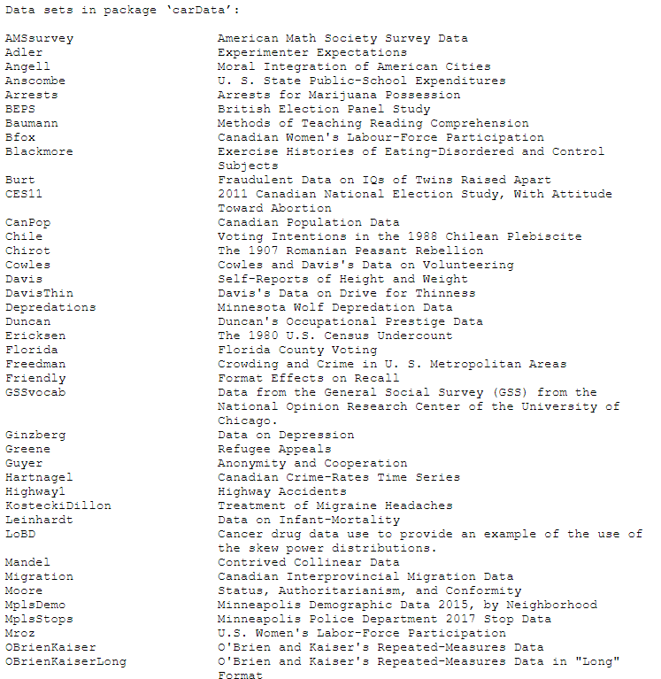
Glimpse of data
Let’s take a look at the inbuilt Salary dataset structure. For that one can utilize the str( ) function or glimpse( ) function from the dplyr library (which is included in the tidyverse library).
glimpse(Salaries)
The dataset includes 397 observations and 6 variables. Rank, discipline and sex are of categorical type while yrs.since.phd, yrs.service and salary are of integer type.
Exploratory data analysis
Before starting to model let’s perform some exploratory data analysis. Let’s see how the salary varies across different ranks. For that, we can plot a bee swarm + box plot combination. From the plot, we can observe that as the rank increases the salary also increases. The mean salary (blue dot) for Male is comparatively higher as compared to female.
ggplot(Salaries, aes(x = sex, y = salary, color = sex)) +
    geom_boxplot()+
    geom_point(size = 2, position = position_jitter(width = 0.2)) +
    stat_summary(fun.y = mean, geom = "point", shape = 20, size = 6, color = "blue")+
    theme_classic() +
    facet_grid(.~rank)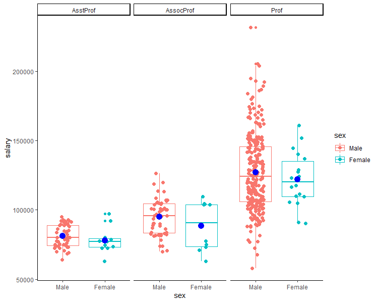
Check gender/sex labels
Before we process for the detailed analysis lets first fit a simple linear regression model where we predict the salary based on gender category. To check the current levels of sex we can use the levels( ) function and supply the column name. By default, the R treats the first level as a reference level (here female).
levels(Salaries$sex)
Fitting a simple linear model
Let’s fit a simple linear regression model with lm( ) function by supplying the formula and dataset.
Formula = salary (~) is predicted by sex
Then print the model summery using the summary( ) function.
lm1 <- lm(salary~sex, data = Salaries)
summary(lm1)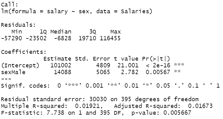
Interpretation of Coefficients
You can observe that the average salary for a female is about 101002 dollars. A male person earns on an average of 14088 dollars more compared to a female person.
Releveling sex variable
We can alter the levels to set male as the reference level. To do so just use the relevel( ) function and supply the column and reference level.
Salaries$sex <- relevel(Salaries$sex, ref = "Male")
levels(Salaries$sex)
Fitting model after releveling
Now if we again fit the model we can now observe a negative sign for female coefficient. A female person earns on an average of 14088 dollars less (115090$ — 14088$) compared to a male person.
lm2 <- lm(salary~sex, data = Salaries)
summary(lm2)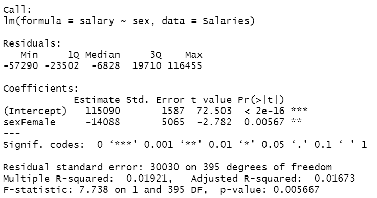
Create a complete model
Let’s fit a multiple linear regression model by supplying all independent variables. The ~ symbol indicates predicted by and dot (.) at the end indicates all independent variables except the dependent variable (salary).
lm_total <- lm(salary~., data = Salaries)
summary(lm_total)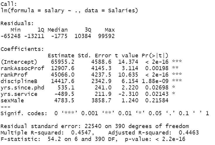
Interpretation of Coefficients
Here we can observe that a person gets an average salary of 65955.2 dollars. The associate professor level is set to the reference level. You can interpret that as ranking increases i.e., from assistant to associate to the professor, the average salary also increases. let’s interpret a continuous variable to say “years of service”. As years of service increases by 1 year, the average salary drops by 489.5 dollars holding all other variables constant.
Similarly, here the diciplineA is the reference category. The discipline B (applied departments) is significantly associated with an average increase of 14417.6 dollars in salary compared to discipline A (theoretical departments) holding other variables at constant.
Stepwise regression
To escape the problem of multicollinearity (correlation among independent variables) and to filter out essential variables/features from a large set of variables, a stepwise regression usually performed. The R language offers forward, backwards and both type of stepwise regression. One can fit a backward stepwise regression using the step( ) function by supplying the initial model object and direction argument. The process starts with initially fitting all the variables and after that, with each iteration, it starts eliminating variables one by one if the variable does not improve the model fit. The AIC metric is used for checking model fit improvement.
step(lm_total, direction = "backward")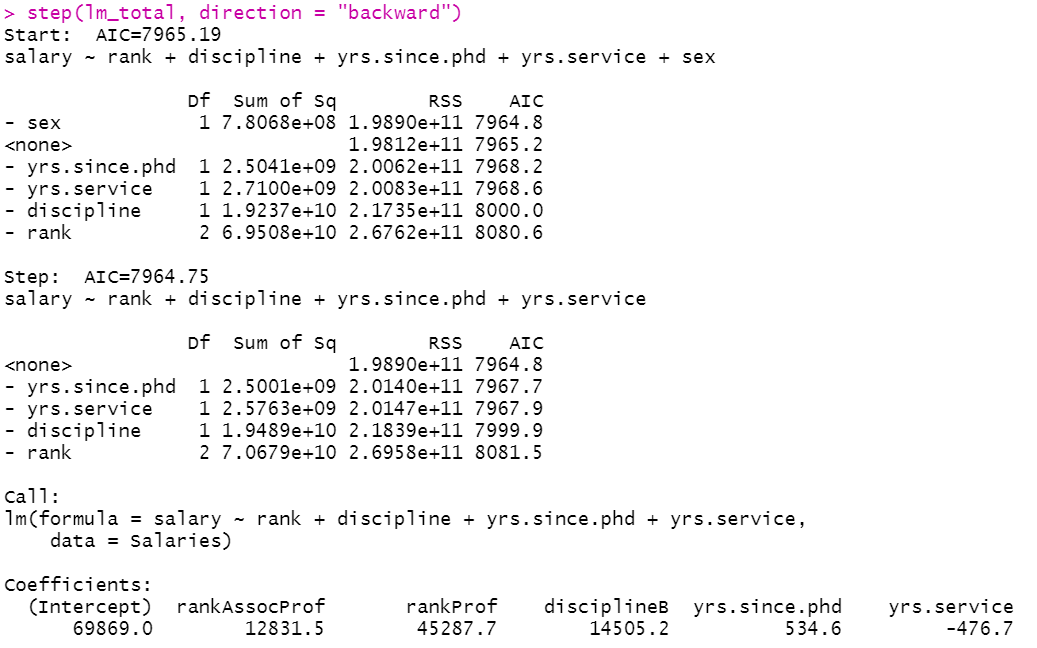
Here, you can see that it eliminated the sex variable from the model but it hardly caused any improvement in the AIC value.
Fitting the improved model
Now, let’s refit the model with the best model variables suggested by the stepwise process.
lm_step_backward <- lm(formula = salary ~ rank + discipline + yrs.since.phd + yrs.service, data = Salaries)
summary(lm_step_backward)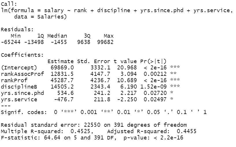
Hypothesis testing
In the next part, we will ask one question and will try to find out the answers by building a hypothesis.
Let’s see the trend of nine months salary over the service period. The best way to do that is by plotting a scatter plot + fitting a trend line.
ggplot(Salaries_mod, aes(x = yrs.service, y = salary)) +
    geom_point()+
    stat_smooth()+
    theme_classic()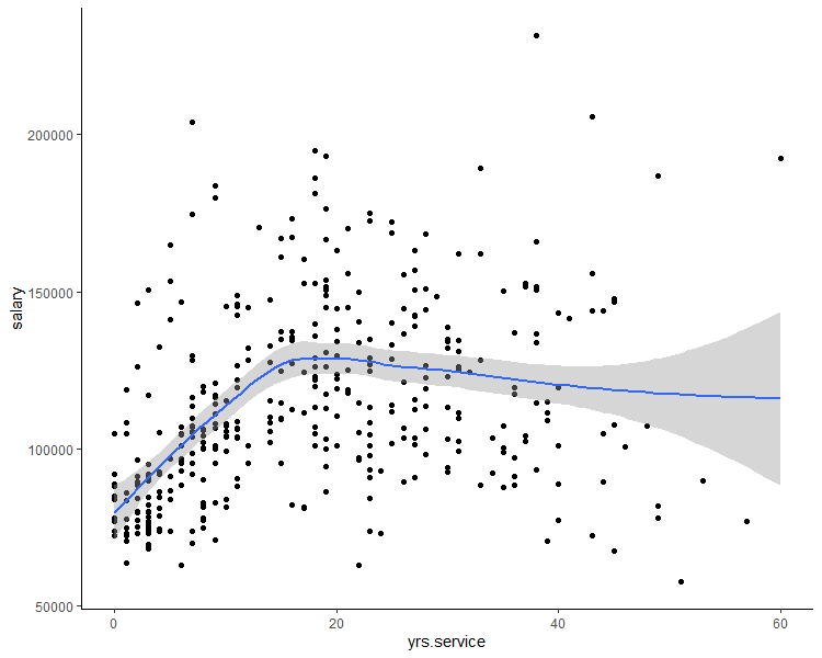
Here, we can observe that up to 20 years of service the salary variable has an increasing trend. After that, the salary shows a decreasing trend.
Converting it to categorical
So we can test one hypothesis that how much on average salary increases or decreases for those having service years of 20–40 years and 40–60 years when compared with 0–20 years (reference). For that purpose, we need to create three categories 0–20, 20–40, 40–60 years where we bin the continuous variable i.e., yrs.service values.
Range estimation
First, we need to identify the service years variable’s data range. To identify the range we can use the range( ) function. You can observe the range is between 0–60 years.
range(Salaries$yrs.service)
Binning yrs.service variable into categories
Lets put the yrs.service variable into three category bins i.e., 0–20, 20–40, 40–60. To do that we can use the mutate( ) function for creating a new column service_time_cat using the case_when( ) function.
Salaries_mod <- Salaries %>%
    mutate(service_time_cat = case_when(
        between(yrs.service, 0, 20)~"upto20",
        between(yrs.service, 20, 40)~"20_40",
        between(yrs.service, 40, 60)~"40_60"))
Converting it to a factor variable
The next step is to convert the new variable into a categorical one. Now, if we check the levels we can observe that the levels are not in proper order.
Salaries_mod$service_time_cat <- as.factor(Salaries_mod$service_time_cat)
levels(Salaries_mod$service_time_cat)
Changing the order of the levels
You can set the level order during categorical conversion or just by using the relevel( ) function. Now the level is in proper order and the reference category is set to “upto20”.
Salaries_mod$service_time_cat <- relevel(Salaries_mod$service_time_cat, ref = "upto20")
levels(Salaries_mod$service_time_cat)
Generating a count table
Let’s see how many unique values each category holds. We can obtain the level count using the table( ) function.
table(Salaries_mod$service_time_cat)
Model Fitting
Let’s refit the model with the newly created categorical variable (service_time_cat).
lm4 <- lm(formula = salary ~ rank + discipline + yrs.since.phd + sex + service_time_cat, data = Salaries_mod)
summary(lm4)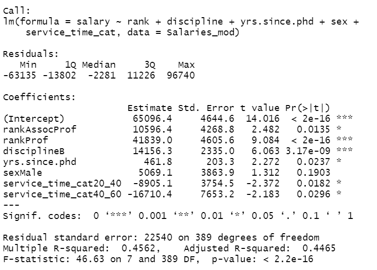
Model interpretation
The model coefficient table showed that as the service time increases the salary decreases (negative coefficients) when compared to the 0–20 years of service. Compared to 0–20 years of service years category, a person is in 20–40 years of service gets on average 8905.1$ less salary, similarly, a person is in 40–60 years service earns 16710.4$ less salary.
Performing a stepwise regression
Next, we can again try to improve the model by performing a backward stepwise regression.
step(lm4, direction = "backward")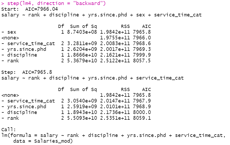
Fitting final model
Let’s fit the final model with stepwise regression suggestion.
lm5 <- lm(formula = salary ~ rank + discipline + yrs.since.phd + service_time_cat,
           data = Salaries_mod)
summary(lm5)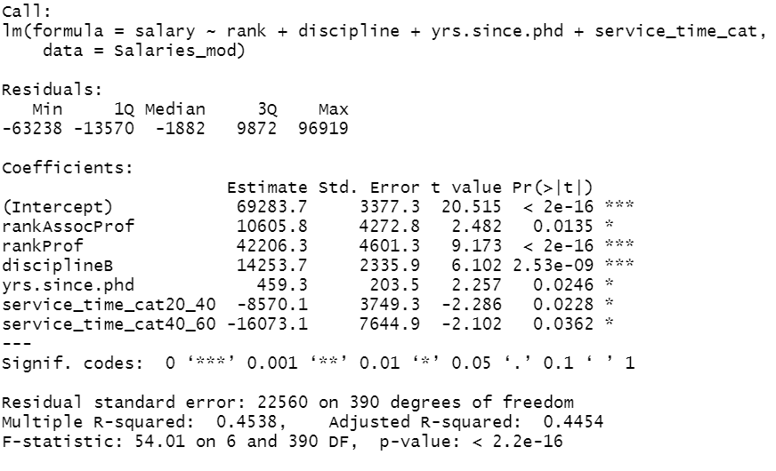
Making result tidy
Sometimes we need the model results in a tidy format so that we can perform certain manipulation on the estimate table. You can convert a model result table into a tidy format using the tidy( ) function from the broom package.
tidy(lm5)
ANOVA analysis
In scenarios where your categorical variables have more than two levels, the interpretation gets complicated. So one can better understand the relationship between independent and dependent variables by performing an anova analysis by supplying the trained model object into the anova( ) function.
The anova analysis result revealed that rank, discipline and service_time_cat variables are significantly associated with the variation in salary (p-values<0.10).
anova(lm5)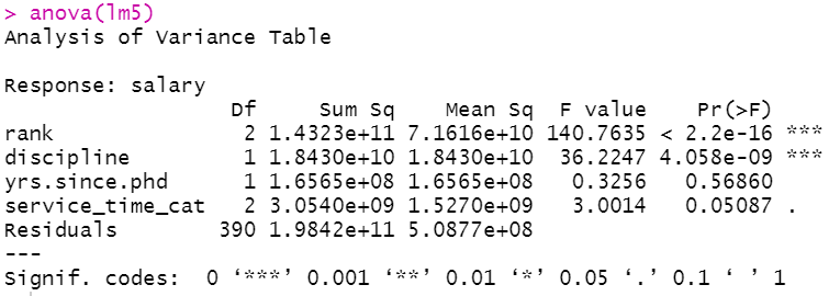
The Multiple Linear regression is still a vastly popular ML algorithm (for regression task) in the STEM research domain. It is still very easy to train and interpret, compared to many sophisticated and complex black-box models.
I hope you learned something new. See you next time!
Featured Image Credit: Photo by Rahul Pandit on Unsplash
References
[1] Fox J. and Weisberg, S. (2019) An R Companion to Applied Regression, Third Edition, Sage.


